Note: This document contains code needed for each part of the Starter Analysis exercise for the MADA Spring 2026 course. Each part is listed under its corresponding part name. As a disclaimer, AI was used for code brevity and assistance in fixing errors in code. Cmd + option + I was used to create chunks for code sections (mac option).
Part 1
Package loading and install
# install dslabs package (run once in the console if not already installed)# install.packages("dslabs")# load required packages# tidyverse added for later steps with data processinglibrary("dslabs")
Warning: package 'dslabs' was built under R version 4.5.2
library("tidyverse")
Warning: package 'ggplot2' was built under R version 4.5.2
Warning: package 'tibble' was built under R version 4.5.2
Warning: package 'tidyr' was built under R version 4.5.2
Warning: package 'readr' was built under R version 4.5.2
Warning: package 'purrr' was built under R version 4.5.2
── Attaching core tidyverse packages ──────────────────────── tidyverse 2.0.0 ──
✔ dplyr     1.1.4     ✔ readr     2.1.6
✔ forcats   1.0.1     ✔ stringr   1.6.0
✔ ggplot2   4.0.1     ✔ tibble    3.3.1
✔ lubridate 1.9.4     ✔ tidyr     1.3.2
✔ purrr     1.2.1
── Conflicts ────────────────────────────────────────── tidyverse_conflicts() ──
✖ dplyr::filter() masks stats::filter()
✖ dplyr::lag()    masks stats::lag()
ℹ Use the conflicted package (<http://conflicted.r-lib.org/>) to force all conflicts to become errors
Show dataset structure
# only run the next command interactively, not in a script# help(gapminder)# get an overview of data structurestr(gapminder)
'data.frame':   10545 obs. of  9 variables:
 $ country         : Factor w/ 185 levels "Albania","Algeria",..: 1 2 3 4 5 6 7 8 9 10 ...
 $ year            : int  1960 1960 1960 1960 1960 1960 1960 1960 1960 1960 ...
 $ infant_mortality: num  115.4 148.2 208 NA 59.9 ...
 $ life_expectancy : num  62.9 47.5 36 63 65.4 ...
 $ fertility       : num  6.19 7.65 7.32 4.43 3.11 4.55 4.82 3.45 2.7 5.57 ...
 $ population      : num  1636054 11124892 5270844 54681 20619075 ...
 $ gdp             : num  NA 1.38e+10 NA NA 1.08e+11 ...
 $ continent       : Factor w/ 5 levels "Africa","Americas",..: 4 1 1 2 2 3 2 5 4 3 ...
 $ region          : Factor w/ 22 levels "Australia and New Zealand",..: 19 11 10 2 15 21 2 1 22 21 ...
# get a summary of datasummary(gapminder)
                country           year      infant_mortality life_expectancy
 Albania            :   57   Min.   :1960   Min.   :  1.50   Min.   :13.20
 Algeria            :   57   1st Qu.:1974   1st Qu.: 16.00   1st Qu.:57.50
 Angola             :   57   Median :1988   Median : 41.50   Median :67.54
 Antigua and Barbuda:   57   Mean   :1988   Mean   : 55.31   Mean   :64.81
 Argentina          :   57   3rd Qu.:2002   3rd Qu.: 85.10   3rd Qu.:73.00
 Armenia            :   57   Max.   :2016   Max.   :276.90   Max.   :83.90
 (Other)            :10203                  NA's   :1453
   fertility       population             gdp               continent
 Min.   :0.840   Min.   :3.124e+04   Min.   :4.040e+07   Africa  :2907
 1st Qu.:2.200   1st Qu.:1.333e+06   1st Qu.:1.846e+09   Americas:2052
 Median :3.750   Median :5.009e+06   Median :7.794e+09   Asia    :2679
 Mean   :4.084   Mean   :2.701e+07   Mean   :1.480e+11   Europe  :2223
 3rd Qu.:6.000   3rd Qu.:1.523e+07   3rd Qu.:5.540e+10   Oceania : 684
 Max.   :9.220   Max.   :1.376e+09   Max.   :1.174e+13
 NA's   :187     NA's   :185         NA's   :2972
             region
 Western Asia   :1026
 Eastern Africa : 912
 Western Africa : 912
 Caribbean      : 741
 South America  : 684
 Southern Europe: 684
 (Other)        :5586
# determine the type of object gapminder isclass(gapminder)
[1] "data.frame"
Data processing
Process Africa subset
# subset gapminder data to rows where continent is "Africa"africadata <- gapminder[gapminder$continent =="Africa", ]# inspect structure (should show 2907 observations; troubleshoot if not)str(africadata)
'data.frame':   2907 obs. of  9 variables:
 $ country         : Factor w/ 185 levels "Albania","Algeria",..: 2 3 18 22 26 27 29 31 32 33 ...
 $ year            : int  1960 1960 1960 1960 1960 1960 1960 1960 1960 1960 ...
 $ infant_mortality: num  148 208 187 116 161 ...
 $ life_expectancy : num  47.5 36 38.3 50.3 35.2 ...
 $ fertility       : num  7.65 7.32 6.28 6.62 6.29 6.95 5.65 6.89 5.84 6.25 ...
 $ population      : num  11124892 5270844 2431620 524029 4829291 ...
 $ gdp             : num  1.38e+10 NA 6.22e+08 1.24e+08 5.97e+08 ...
 $ continent       : Factor w/ 5 levels "Africa","Americas",..: 1 1 1 1 1 1 1 1 1 1 ...
 $ region          : Factor w/ 22 levels "Australia and New Zealand",..: 11 10 20 17 20 5 10 20 10 10 ...
# check summary statistics
summary(africadata)
         country          year      infant_mortality life_expectancy
 Algeria     :  57   Min.   :1960   Min.   : 11.40   Min.   :13.20
 Angola      :  57   1st Qu.:1974   1st Qu.: 62.20   1st Qu.:48.23
 Benin       :  57   Median :1988   Median : 93.40   Median :53.98
 Botswana    :  57   Mean   :1988   Mean   : 95.12   Mean   :54.38
 Burkina Faso:  57   3rd Qu.:2002   3rd Qu.:124.70   3rd Qu.:60.10
 Burundi     :  57   Max.   :2016   Max.   :237.40   Max.   :77.60
 (Other)     :2565                  NA's   :226
   fertility       population             gdp               continent
 Min.   :1.500   Min.   :    41538   Min.   :4.659e+07   Africa  :2907
 1st Qu.:5.160   1st Qu.:  1605232   1st Qu.:8.373e+08   Americas:   0
 Median :6.160   Median :  5570982   Median :2.448e+09   Asia    :   0
 Mean   :5.851   Mean   : 12235961   Mean   :9.346e+09   Europe  :   0
 3rd Qu.:6.860   3rd Qu.: 13888152   3rd Qu.:6.552e+09   Oceania :   0
 Max.   :8.450   Max.   :182201962   Max.   :1.935e+11
 NA's   :51      NA's   :51          NA's   :637
                       region
 Eastern Africa           :912
 Western Africa           :912
 Middle Africa            :456
 Northern Africa          :342
 Southern Africa          :285
 Australia and New Zealand:  0
 (Other)                  :  0
# keep only infant_mortality and life_expectancyafrica_infant_mortality <- africadata[, c("infant_mortality", "life_expectancy")]# keep only population and life_expectancyafrica_population <- africadata[, c("population", "life_expectancy")]# inspect structure + summariesstr(africa_infant_mortality)
'data.frame':   2907 obs. of  2 variables:
 $ infant_mortality: num  148 208 187 116 161 ...
 $ life_expectancy : num  47.5 36 38.3 50.3 35.2 ...
summary(africa_infant_mortality)
 infant_mortality life_expectancy
 Min.   : 11.40   Min.   :13.20
 1st Qu.: 62.20   1st Qu.:48.23
 Median : 93.40   Median :53.98
 Mean   : 95.12   Mean   :54.38
 3rd Qu.:124.70   3rd Qu.:60.10
 Max.   :237.40   Max.   :77.60
 NA's   :226
str(africa_population)
'data.frame':   2907 obs. of  2 variables:
 $ population     : num  11124892 5270844 2431620 524029 4829291 ...
 $ life_expectancy: num  47.5 36 38.3 50.3 35.2 ...
summary(africa_population)
   population        life_expectancy
 Min.   :    41538   Min.   :13.20
 1st Qu.:  1605232   1st Qu.:48.23
 Median :  5570982   Median :53.98
 Mean   : 12235961   Mean   :54.38
 3rd Qu.: 13888152   3rd Qu.:60.10
 Max.   :182201962   Max.   :77.60
 NA's   :51
How to plot the data
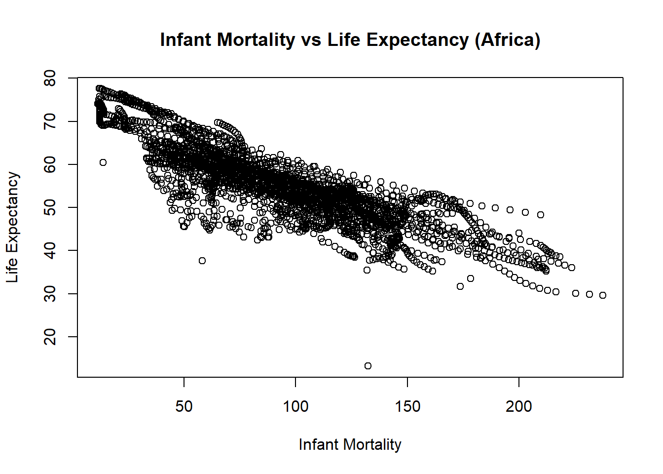
# life expectancy vs infant mortality (points)plot(x = africa_infant_mortality$infant_mortality,y = africa_infant_mortality$life_expectancy,xlab ="Infant Mortality",ylab ="Life Expectancy",main ="Infant Mortality vs Life Expectancy (Africa)")
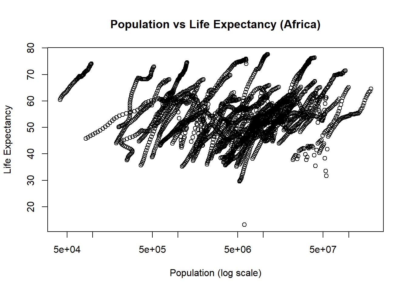
# life expectancy vs population (points) with log-scaled x-axisplot(x = africa_population$population,y = africa_population$life_expectancy,xlab ="Population (log scale)",ylab ="Life Expectancy",main ="Population vs Life Expectancy (Africa)",log ="x")
The infant mortality plot shows a negative correlation with life expectancy, while the population plot shows a general positive relationship. The plots appear to in a streaking form because individual countries are counted across multiple points. In the population vs life expectancy (Africa) plot, we can see that for individual country populations, as population increases, so does life expectancy.
# count missing infant_mortality values for each yeartapply(africadata$infant_mortality, africadata$year, function(x) sum(is.na(x)))
# subset to year 2000africa_2000 <- africadata[africadata$year ==2000, ]str(africa_2000)
'data.frame':   51 obs. of  9 variables:
 $ country         : Factor w/ 185 levels "Albania","Algeria",..: 2 3 18 22 26 27 29 31 32 33 ...
 $ year            : int  2000 2000 2000 2000 2000 2000 2000 2000 2000 2000 ...
 $ infant_mortality: num  33.9 128.3 89.3 52.4 96.2 ...
 $ life_expectancy : num  73.3 52.3 57.2 47.6 52.6 46.7 54.3 68.4 45.3 51.5 ...
 $ fertility       : num  2.51 6.84 5.98 3.41 6.59 7.06 5.62 3.7 5.45 7.35 ...
 $ population      : num  31183658 15058638 6949366 1736579 11607944 ...
 $ gdp             : num  5.48e+10 9.13e+09 2.25e+09 5.63e+09 2.61e+09 ...
 $ continent       : Factor w/ 5 levels "Africa","Americas",..: 1 1 1 1 1 1 1 1 1 1 ...
 $ region          : Factor w/ 22 levels "Australia and New Zealand",..: 11 10 20 17 20 5 10 20 10 10 ...
summary(africa_2000)
         country        year      infant_mortality life_expectancy
 Algeria     : 1   Min.   :2000   Min.   : 12.30   Min.   :37.60
 Angola      : 1   1st Qu.:2000   1st Qu.: 60.80   1st Qu.:51.75
 Benin       : 1   Median :2000   Median : 80.30   Median :54.30
 Botswana    : 1   Mean   :2000   Mean   : 78.93   Mean   :56.36
 Burkina Faso: 1   3rd Qu.:2000   3rd Qu.:103.30   3rd Qu.:60.00
 Burundi     : 1   Max.   :2000   Max.   :143.30   Max.   :75.00
 (Other)     :45
   fertility       population             gdp               continent
 Min.   :1.990   Min.   :    81154   Min.   :2.019e+08   Africa  :51
 1st Qu.:4.150   1st Qu.:  2304687   1st Qu.:1.274e+09   Americas: 0
 Median :5.550   Median :  8799165   Median :3.238e+09   Asia    : 0
 Mean   :5.156   Mean   : 15659800   Mean   :1.155e+10   Europe  : 0
 3rd Qu.:5.960   3rd Qu.: 17391242   3rd Qu.:8.654e+09   Oceania : 0
 Max.   :7.730   Max.   :122876723   Max.   :1.329e+11

                       region
 Eastern Africa           :16
 Western Africa           :16
 Middle Africa            : 8
 Northern Africa          : 6
 Southern Africa          : 5
 Australia and New Zealand: 0
 (Other)                  : 0
fit1 <-lm(life_expectancy ~ infant_mortality, data = africa_2000)summary(fit1)
Call:
lm(formula = life_expectancy ~ infant_mortality, data = africa_2000)

Residuals:
     Min       1Q   Median       3Q      Max
-22.6651  -3.7087   0.9914   4.0408   8.6817

Coefficients:
                 Estimate Std. Error t value Pr(>|t|)
(Intercept)      71.29331    2.42611  29.386  < 2e-16 ***
infant_mortality -0.18916    0.02869  -6.594 2.83e-08 ***
---
Signif. codes:  0 '***' 0.001 '**' 0.01 '*' 0.05 '.' 0.1 ' ' 1

Residual standard error: 6.221 on 49 degrees of freedom
Multiple R-squared:  0.4701,    Adjusted R-squared:  0.4593
F-statistic: 43.48 on 1 and 49 DF,  p-value: 2.826e-08
fit2 <-lm(life_expectancy ~ population, data = africa_2000)summary(fit2)
Call:
lm(formula = life_expectancy ~ population, data = africa_2000)

Residuals:
    Min      1Q  Median      3Q     Max
-18.429  -4.602  -2.568   3.800  18.802

Coefficients:
             Estimate Std. Error t value Pr(>|t|)
(Intercept) 5.593e+01  1.468e+00  38.097   <2e-16 ***
population  2.756e-08  5.459e-08   0.505    0.616
---
Signif. codes:  0 '***' 0.001 '**' 0.01 '*' 0.05 '.' 0.1 ' ' 1

Residual standard error: 8.524 on 49 degrees of freedom
Multiple R-squared:  0.005176,  Adjusted R-squared:  -0.01513
F-statistic: 0.2549 on 1 and 49 DF,  p-value: 0.6159
Fit1 shows that infant mortality shows a statistically significant negative relationship with life expectancy(p = 2.83^-08), explaining approximately 47% of the variation in life expectancy among African countries in 2000. In contrast, population size shows no significant association with life expectancy (p = 0.616). The model fit is also highly significant with a prediction error rate of 6.221 years (F= 43.48, p= 2.825^-08).
Fit2 indicates that there is no statistically significant relationship between population size and life expectancy (estimate =2.756^-08; p=0.616). The model is not significant and does not explain the variation in life expectancy (R2= 0.005176; adjusted value of -0.01513; F= 0.2549, p= 0.6159). Predictor error is large for this dataset at 8.524 years.
The following section contributed by Elle Adams
#Need dplyr to pipe data library(dplyr)library(tidyverse)library(dslabs)#New dslabs data set - murders (I like true crime)#overview of structurestr(murders)
    state               abb                      region     population
 Length:51          Length:51          Northeast    : 9   Min.   :  563626
 Class :character   Class :character   South        :17   1st Qu.: 1696962
 Mode  :character   Mode  :character   North Central:12   Median : 4339367
                                       West         :13   Mean   : 6075769
                                                          3rd Qu.: 6636084
                                                          Max.   :37253956
     total
 Min.   :   2.0
 1st Qu.:  24.5
 Median :  97.0
 Mean   : 184.4
 3rd Qu.: 268.0
 Max.   :1257.0
#create new column total/population * 100000 to get number of murders per 100,000 people for each state (how it's typically expressed)murders <- murders %>%mutate(murder_rate = (total/population)*100000)#check new structure str(murders)
'data.frame':   51 obs. of  6 variables:
 $ state      : chr  "Alabama" "Alaska" "Arizona" "Arkansas" ...
 $ abb        : chr  "AL" "AK" "AZ" "AR" ...
 $ region     : Factor w/ 4 levels "Northeast","South",..: 2 4 4 2 4 4 1 2 2 2 ...
 $ population : num  4779736 710231 6392017 2915918 37253956 ...
 $ total      : num  135 19 232 93 1257 ...
 $ murder_rate: num  2.82 2.68 3.63 3.19 3.37 ...
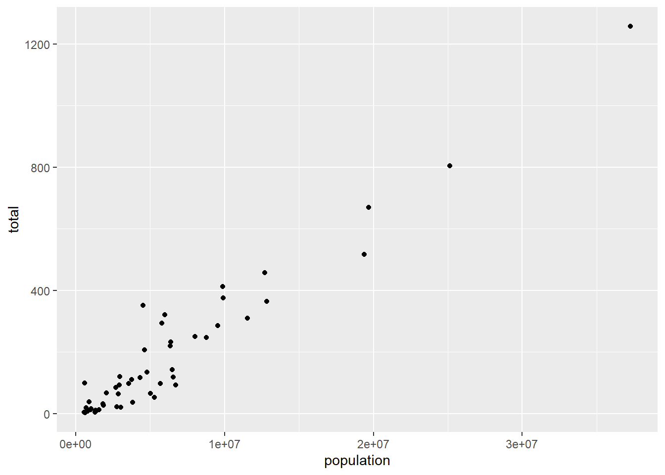
#Question 1 - what is the relationship between population and number of murders? hypothesis - more people = more murder#Plot population (x) vs total (y)ggplot(murders, (aes(x = population, y = total))) +geom_point()
#Fit with total as outcome and population as predictortotal_vs_pop <-lm(total ~ population, data = murders)#See the fitsummary(total_vs_pop)
Call:
lm(formula = total ~ population, data = murders)

Residuals:
     Min       1Q   Median       3Q      Max
-112.889  -25.656   -3.687   25.505  217.780

Coefficients:
              Estimate Std. Error t value Pr(>|t|)
(Intercept) -1.713e+01  1.198e+01   -1.43    0.159
population   3.316e-05  1.315e-06   25.23   <2e-16 ***
---
Signif. codes:  0 '***' 0.001 '**' 0.01 '*' 0.05 '.' 0.1 ' ' 1

Residual standard error: 63.77 on 49 degrees of freedom
Multiple R-squared:  0.9285,    Adjusted R-squared:  0.9271
F-statistic: 636.5 on 1 and 49 DF,  p-value: < 2.2e-16
What I found: There is a strong, positive correlation between population and total number of murders (R-squared = 0.9271) and this is significant (p-value = 2e-16, much smaller than 0.05). This is confirmed visually by the graph.
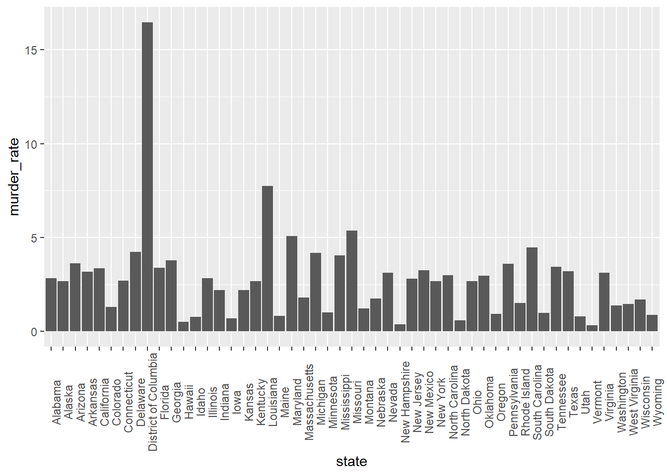
#Question 2 - which state has the most murders per 100,000 people? hypothesis - new york #Figure showing the number of murders per 100,000 people for each stateggplot(murders, aes(x = state, y = murder_rate)) +geom_col() +theme(axis.text.x =element_text(angle =90))
#What is murder rate for DC? (Alphabetically row number 9)slice(murders, 9)
                 state abb region population total murder_rate
1 District of Columbia  DC  South     601723    99    16.45275
Using this figure, I can see that I was incorrect in my hypothesis - DC actually as the highest murder rate, at 16.45275 murders per 100,000 people.