Presenting Data on Netflix Viewership

I chose to recreate the figures from Netflix’s What We Watched the Second Half of 2025, which can be found here. The report includes data on the most popular shows and movies on Netflix in the second half of 2025, as well as insights into viewership trends and run times. The data were separated by Movie and Shows, and I liked the aesthetic of the original report.

Loading and checking Netflix data

# install packages if not already installed (run once in the console)
# load required packages
library("readr")
Warning: package 'readr' was built under R version 4.5.2
library("stringr")
library("here")
here() starts at /Users/nalanyrichardson/Downloads/MADA/Portfolio
library("janitor") 

Attaching package: 'janitor'
The following objects are masked from 'package:stats':

    chisq.test, fisher.test
library("dplyr")

Attaching package: 'dplyr'
The following objects are masked from 'package:stats':

    filter, lag
The following objects are masked from 'package:base':

    intersect, setdiff, setequal, union
library("ggplot2")
Warning: package 'ggplot2' was built under R version 4.5.2
library("scales")

Attaching package: 'scales'
The following object is masked from 'package:readr':

    col_factor
library("skimr")
Warning: package 'skimr' was built under R version 4.5.2
# read in the data
netflix_shows  <- readxl::read_excel("netflix-engagement.xlsx", sheet = "Shows",  skip = 5)
Warning: Expecting numeric in G7752 / R7752C7: got '*'
netflix_movies <- readxl::read_excel("netflix-engagement.xlsx", sheet = "Movies", skip = 5)
Warning: Expecting numeric in G8730 / R8730C7: got '*'

Doublecheck data structure

Now we should take a look at what the data actually looks like.

# get an overview of data structure
glimpse(netflix_shows)
Rows: 7,748
Columns: 6
$ Title                 <chr> "Wednesday: Season 2", "Stranger Things 5", "UNT…
$ `Available Globally?` <chr> "Yes", "Yes", "Yes", "Yes", "Yes", "Yes", "Yes",…
$ `Release Date`        <chr> "2025-08-06", "2025-11-26", "2025-07-17", "2025-…
$ `Hours Viewed`        <dbl> 964100000, 879700000, 451600000, 484300000, 3860…
$ Runtime               <chr> "7:47", "*", "4:52", "6:08", "6:49", "7:27", "4:…
$ Views                 <dbl> 123900000, 93500000, 92800000, 79000000, 5660000…
glimpse(netflix_movies)
Rows: 8,726
Columns: 6
$ Title                 <chr> "KPop Demon Hunters", "Happy Gilmore 2", "Franke…
$ `Available Globally?` <chr> "Yes", "Yes", "Yes", "Yes", "Yes", "Yes", "Yes",…
$ `Release Date`        <chr> "2025-06-20", "2025-07-25", "2025-11-07", "2025-…
$ `Hours Viewed`        <dbl> 802600000, 265700000, 247300000, 162200000, 1453…
$ Runtime               <chr> "1:40", "1:58", "2:32", "1:53", "1:47", "1:35", …
$ Views                 <dbl> 481600000, 135100000, 97600000, 86100000, 815000…

The data were already cleaned before running, with the exception of the column headers being in row 6, so I can skip cleaning. There were a couple rows with * in the Runtime column, but they won’t affect the structure of the data so we can ignore this.

Recreating the figures

# load Most Watched Movies figure
knitr::include_graphics("assets/most-watched-movies.png")

Prompt 1: I want to recreate most-watched-movies.png graphic figure. I need to compose a single figure where red top banner with NETFLIX in small bold white text in the top left corner and MOST-WATCHED MOVIES in large black bold text with MOVIES under MOST-WATCHED text. I want the 10 horizontal rows with the highest views_ value to be white filled with a small bit of space between each row, and the name of the corresponding Title to be inside the row along with its numerical rank (e.g., 1 KPOP DEMON HUNTERS) with the views_m rounded value label displayed at the end of the row outside of the row in bold black text (e.g., 482,000,000 would be 482M). the .png is stored as assets/most-watched-movies.png

Prompt 2: The first image did not have a red background, text was not truly bolded, and the numerical rank was in a black box. Now I Please don’t judge the prompting language. I found if I use less filler words, delineators, etc… then Chatgpt will be less verbose and will give chunks without having to push over and over…

Some edits were made without the use of AI, like fixing the figure width/height since it looked smushed when rendered. There may be other ways to fix this, but I just found a size I was happy with.

top_10_movie <- netflix_movies |>
  dplyr::arrange(dplyr::desc(Views)) |>
  dplyr::slice_head(n = 10) |>
  dplyr::mutate(
    rank = dplyr::row_number(),
    views_m = Views / 1e6,
    views_label = paste0(round(views_m), "M"),
    Title = factor(Title, levels = rev(Title))
  ) |>
  dplyr::select(rank, Title, views_m, views_label)
library(dplyr)
library(ggplot2)
library(scales)
library(showtext)
Loading required package: sysfonts
Loading required package: showtextdb
library(sysfonts)

font_add_google("Anton", "anton")
showtext_auto()

# ---- data prep ----
plot_df <- top_10_movie |>
  mutate(
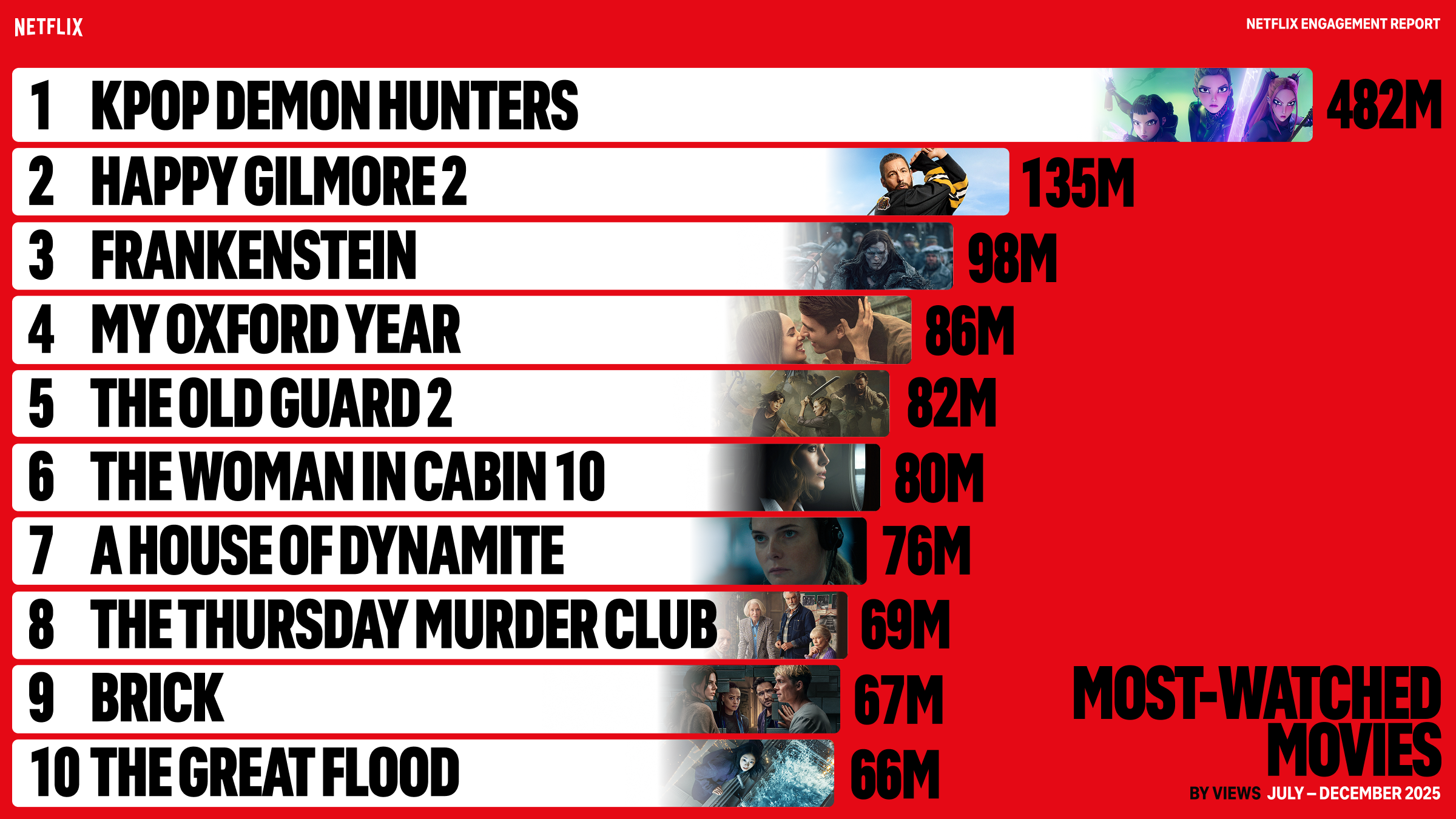
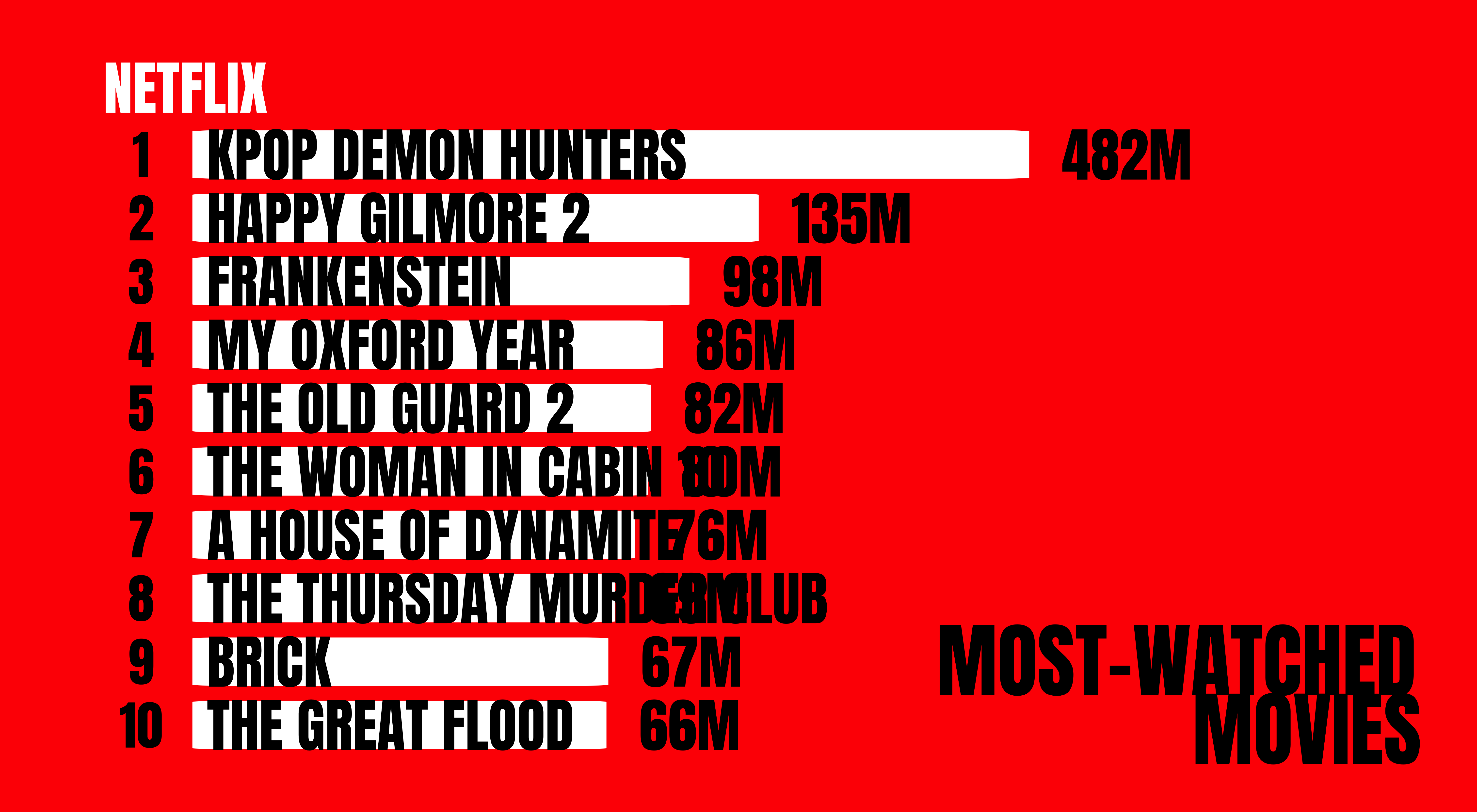
    Title = ifelse(rank == 10, "THE GREAT FLOOD", as.character(Title)),
    title_upper = toupper(Title),
    views_m = as.numeric(views_m),
    # compress the range so smaller titles show more difference
    bar_len = scales::rescale(log10(views_m), to = c(0.55, 1.00)),
    # y positions so rank 1 is at top
    y = rev(rank)
  )

# ---- helper: true rounded-corner rectangle as polygon ----
rounded_rect_df <- function(id, xmin, xmax, ymin, ymax, r = 0.03, n = 25) {
  r <- min(r, (xmax - xmin)/2, (ymax - ymin)/2)

  arc <- function(cx, cy, start, end) {
    t <- seq(start, end, length.out = n)
    tibble(x = cx + r * cos(t), y = cy + r * sin(t))
  }

  top    <- tibble(x = seq(xmax - r, xmin + r, length.out = 2), y = ymax)
  left   <- tibble(x = xmin, y = seq(ymax - r, ymin + r, length.out = 2))
  bottom <- tibble(x = seq(xmin + r, xmax - r, length.out = 2), y = ymin)
  right  <- tibble(x = xmax, y = seq(ymin + r, ymax - r, length.out = 2))

  pts <- bind_rows(
    arc(xmax - r, ymax - r, 0,  pi/2),       # top-right
    top,
    arc(xmin + r, ymax - r, pi/2, pi),       # top-left
    left,
    arc(xmin + r, ymin + r, pi, 3*pi/2),     # bottom-left
    bottom,
    arc(xmax - r, ymin + r, 3*pi/2, 2*pi),   # bottom-right
    right
  )

  pts |> mutate(group = id)
}

# build polygon data for all 10 bars
bar_poly <- plot_df |>
  rowwise() |>
  do(rounded_rect_df(
    id   = .$rank,
    xmin = 0.10,
    xmax = .$bar_len,
    ymin = .$y - 0.45,
    ymax = .$y + 0.45,
    r    = 0.03,   # increase for more rounding, decrease for less
    n    = 25
  )) |>
  ungroup()

# ---- plot ----
most_watched_movies_plot <- ggplot() +
  coord_cartesian(xlim = c(0, 1.35), ylim = c(0.5, 11.5), clip = "off") +
  theme_void() +
  theme(
    panel.background = element_rect(fill = "red", color = NA),
    plot.background  = element_rect(fill = "red", color = NA),
    plot.margin = margin(12, 25, 10, 15)
  ) +
  # rounded bars
  geom_polygon(
    data = bar_poly,
    aes(x = x, y = y, group = group),
    fill = "white", color = "red", linewidth = 2
  ) +
  # rank numbers (no box)
  geom_text(
    data = plot_df,
    aes(x = 0.05, y = y, label = rank),
    family = "anton", fontface = "bold",
    color = "black", size = 9
  ) +
  # titles
  geom_text(
    data = plot_df,
    aes(x = 0.12, y = y, label = title_upper),
    hjust = 0,
    family = "anton", fontface = "bold",
    color = "black", size = 10
  ) +
  # value labels beside bar end
  geom_text(
    data = plot_df,
    aes(x = bar_len + 0.03, y = y, label = views_label),
    hjust = 0,
    family = "anton", fontface = "bold",
    color = "black", size = 10
  ) +
  # NETFLIX top-left
  annotate(
    "text", x = 0.01, y = 11.45, label = "NETFLIX",
    hjust = 0, vjust = 1,
    family = "anton", fontface = "bold",
    color = "white", size = 10
  ) +
  # bottom-right block
  annotate(
  "text", x = Inf, y = -Inf, label = "MOST-WATCHED\nMOVIES",
  hjust = 1.02, vjust = -0.2,
  family = "anton", fontface = "bold",
  color = "black", size = 14, lineheight = 0.7
)
most_watched_movies_plot

As we can see, the trends are identical to the original figure. Aesthetically, there were no images available in their zip file to place into the bars, and I couldn’t manage to get the numerical rankings into the white box on my own.

For tables, I wanted to create a top 20 for overall titles, regardless of type. I also wanted to see how total views and hours compared to each other. There are inherent differences in show and movie format, since a movie is typically <3 hours but a show can have >8 hours in a given season, and some individuals may rewatch a movie/show and contribute more hours than total views.

For prompts, I asked Chatgpt to create a table formatted by Rank Type Title Views Hours Viewed Available Globally? with the top 20 overall titles by views, and then to format that table with gt and make sure there was a hover effect on the rows, and to make movie rows light blue and show rows like orange to better showcase differences. It did try to create funky tables with packages no longer functional in my current version of R. The table took the longest time and kept crashing my LLM.

top20_overall <- dplyr::bind_rows(
  netflix_movies |> dplyr::mutate(Type = "Movie"),
  netflix_shows  |> dplyr::mutate(Type = "Show")
) |>
  dplyr::arrange(dplyr::desc(Views)) |>
  dplyr::slice_head(n = 20) |>
  dplyr::mutate(
    Rank = dplyr::row_number(),
    Views_M = Views / 1e6,
    Views_Label = paste0(round(Views_M), "M")
  ) |>
  dplyr::select(
    Rank, Type, Title,
    `Available Globally?`, `Release Date`,
    `Hours Viewed`, Views_Label
  )

top20_overall
# A tibble: 20 × 7
    Rank Type  Title         `Available Globally?` `Release Date` `Hours Viewed`
   <int> <chr> <chr>         <chr>                 <chr>                   <dbl>
 1     1 Movie KPop Demon H… Yes                   2025-06-20          802600000
 2     2 Movie Happy Gilmor… Yes                   2025-07-25          265700000
 3     3 Show  Wednesday: S… Yes                   2025-08-06          964100000
 4     4 Movie Frankenstein  Yes                   2025-11-07          247300000
 5     5 Show  Stranger Thi… Yes                   2025-11-26          879700000
 6     6 Show  UNTAMED: Sea… Yes                   2025-07-17          451600000
 7     7 Movie My Oxford Ye… Yes                   2025-08-01          162200000
 8     8 Movie The Old Guar… Yes                   2025-07-02          145300000
 9     9 Movie The Woman in… Yes                   2025-10-10          127300000
10    10 Show  Squid Game: … Yes                   2025-06-27          484300000
11    11 Movie A HOUSE OF D… Yes                   2025-10-24          144800000
12    12 Movie The Thursday… Yes                   2025-08-28          137500000
13    13 Movie Brick         Yes                   2025-07-10          112200000
14    14 Movie The Great Fl… Yes                   2025-12-19          120000000
15    15 Movie Madea’s Dest… Yes                   2025-07-11          104500000
16    16 Movie The Wrong Pa… Yes                   2025-09-12          103400000
17    17 Movie Unknown Numb… Yes                   2025-08-29           90000000
18    18 Show  Stranger Thi… Yes                   2016-07-15          386000000
19    19 Movie Wake Up Dead… Yes                   2025-12-12          136900000
20    20 Show  Monster: The… Yes                   2025-10-03          415600000
# ℹ 1 more variable: Views_Label <chr>
top20_table <- top20_overall |>
  dplyr::select(
    Rank, Type, Title, Views_Label, `Hours Viewed`, `Available Globally?`
  ) |>
  gt::gt() |>
  gt::cols_label(
    Rank = "Rank",
    Type = "Type",
    Title = "Title",
    Views_Label = "Views",
    `Hours Viewed` = "Hours Viewed",
    `Available Globally?` = "Available Globally?"
  ) |>
  gt::fmt_number(
    columns = `Hours Viewed`,
    sep_mark = ",",
    decimals = 0
  ) |>
  gt::cols_align(
    align = "center",
    columns = c(Rank, Type, Views_Label, `Hours Viewed`, `Available Globally?`)
  ) |>
  gt::cols_align(
    align = "left",
    columns = Title
  ) |>
  gt::tab_header(
    title = gt::md("**Top 20 Netflix Titles by Views**"),
    subtitle = "Movies and Shows Engagement July-December 2025"
  ) |>
  gt::tab_style(
    style = gt::cell_text(weight = "bold"),
    locations = gt::cells_column_labels(gt::everything())
  ) |>
  gt::tab_style(
    style = gt::cell_fill(color = "#d9ecff"),
    locations = gt::cells_body(rows = Type == "Movie")
  ) |>
  gt::tab_style(
    style = gt::cell_fill(color = "#ffe6cc"),
    locations = gt::cells_body(rows = Type == "Show")
  ) |>
  gt::tab_options(
    table.additional_css = "
      tr:hover td { 
        background-color: #ffffcc !important; 
      }
    "
  ) |>
  gt::tab_source_note(
    source_note = gt::md("**Source/Credit:** Netflix — *What We Watched: The Second Half of 2025* (Engagement Report).")
  )

top20_table
Top 20 Netflix Titles by Views
Movies and Shows Engagement July-December 2025
Rank Type Title Views Hours Viewed Available Globally?
1 Movie KPop Demon Hunters 482M 802,600,000 Yes
2 Movie Happy Gilmore 2 135M 265,700,000 Yes
3 Show Wednesday: Season 2 124M 964,100,000 Yes
4 Movie Frankenstein 98M 247,300,000 Yes
5 Show Stranger Things 5 94M 879,700,000 Yes
6 Show UNTAMED: Season 1 93M 451,600,000 Yes
7 Movie My Oxford Year 86M 162,200,000 Yes
8 Movie The Old Guard 2 82M 145,300,000 Yes
9 Movie The Woman in Cabin 10 80M 127,300,000 Yes
10 Show Squid Game: Season 3 // 오징어 게임: 시즌 3 79M 484,300,000 Yes
11 Movie A HOUSE OF DYNAMITE 76M 144,800,000 Yes
12 Movie The Thursday Murder Club 69M 137,500,000 Yes
13 Movie Brick 67M 112,200,000 Yes
14 Movie The Great Flood // 대홍수 66M 120,000,000 Yes
15 Movie Madea’s Destination Wedding 60M 104,500,000 Yes
16 Movie The Wrong Paris 58M 103,400,000 Yes
17 Movie Unknown Number: The High School Catfish 57M 90,000,000 Yes
18 Show Stranger Things 57M 386,000,000 Yes
19 Movie Wake Up Dead Man: A Knives Out Mystery 56M 136,900,000 Yes
20 Show Monster: The Ed Gein Story 56M 415,600,000 Yes
Source/Credit: Netflix — What We Watched: The Second Half of 2025 (Engagement Report).

Movies dominated the top 20 overall titles by views (16/20) by both views_m and total views. When looking by hours viewed, the top shows dominated over movies. I had heard of KPop Demon Hunters being trendy, but it is incredible to see how dominant it actually was! For future analyses, it would be interesting to see how international titles and titles not available globally perform in their respective regions. This could possibly inform testers for what content to bring to the US market, considering how well titles like the aforementioned KPop Demon Hunters, as well as Squid Game, and The Great Flood performed.