This data analysis was done using the Provisional COVID-19 Deaths by Race and Hispanic Origin, and Age dataset provided by the NCHS/DVS, which contains data on deaths involving COVID-19, pneumonia, and influenza, categorized by race/age/jurisdiction.
There are 13 columns listed:
Date as of - date of analysis
Start date - first date of data period
End date - last date of data period
State - jurisdiction of occurrence
Age group - age group
Race and Hispanic Origin Group - Race or Hispanic origin group
Pneumonia, Influenza, or COVID-19 deaths - deaths with any of aforementioned codes.
Footnote- suppressed counts (1-9)
Package loading and install
First we need to upload and/or install packages for cleaning our data
# install packages if not already installed (run once in the console)# load required packages# tidyverse added for later steps with data processinglibrary("dslabs")
Warning: package 'dslabs' was built under R version 4.5.2
library("tidyverse")
Warning: package 'ggplot2' was built under R version 4.5.2
Warning: package 'tibble' was built under R version 4.5.2
Warning: package 'tidyr' was built under R version 4.5.2
Warning: package 'readr' was built under R version 4.5.2
Warning: package 'purrr' was built under R version 4.5.2
── Attaching core tidyverse packages ──────────────────────── tidyverse 2.0.0 ──
✔ dplyr     1.1.4     ✔ readr     2.1.6
✔ forcats   1.0.1     ✔ stringr   1.6.0
✔ ggplot2   4.0.1     ✔ tibble    3.3.1
✔ lubridate 1.9.4     ✔ tidyr     1.3.2
✔ purrr     1.2.1
── Conflicts ────────────────────────────────────────── tidyverse_conflicts() ──
✖ dplyr::filter() masks stats::filter()
✖ dplyr::lag()    masks stats::lag()
ℹ Use the conflicted package (<http://conflicted.r-lib.org/>) to force all conflicts to become errors
library("readr")library("stringr")library("here")
here() starts at /Users/nalanyrichardson/Downloads/MADA/Portfolio
library("janitor")
Attaching package: 'janitor'

The following objects are masked from 'package:stats':

    chisq.test, fisher.test
# read in the datacdcdata <-read_csv(here("cdcdata-exercise", "Provisional_COVID-19_Deaths_by_Race_and_Hispanic_Origin,_and_Age_20260211.csv"))
Rows: 6489 Columns: 13
── Column specification ────────────────────────────────────────────────────────
Delimiter: ","
chr (7): Data as of, Start Date, End Date, State, Age group, Race and Hispan...
num (6): COVID-19 Deaths, Total Deaths, Pneumonia Deaths, Pneumonia and COVI...

ℹ Use `spec()` to retrieve the full column specification for this data.
ℹ Specify the column types or set `show_col_types = FALSE` to quiet this message.
Show dataset structure
Now we should take a look at what the data actually looks like.
# get an overview of data structure# I prefer str() for checking out the data, but I also like glimpse() for very rote summaries where you can determine characteristics.We can run all of them and see what we get, and then just choose whatever we'd like.str(cdcdata)
spc_tbl_ [6,489 × 13] (S3: spec_tbl_df/tbl_df/tbl/data.frame)
 $ Data as of                              : chr [1:6489] "09/27/2023" "09/27/2023" "09/27/2023" "09/27/2023" ...
 $ Start Date                              : chr [1:6489] "01/01/2020" "01/01/2020" "01/01/2020" "01/01/2020" ...
 $ End Date                                : chr [1:6489] "09/23/2023" "09/23/2023" "09/23/2023" "09/23/2023" ...
 $ State                                   : chr [1:6489] "United States" "United States" "United States" "United States" ...
 $ Age group                               : chr [1:6489] "All Ages" "All Ages" "Under 1 year" "0-17 years" ...
 $ Race and Hispanic Origin Group          : chr [1:6489] "Total Deaths" "Non-Hispanic White" "Non-Hispanic White" "Non-Hispanic White" ...
 $ COVID-19 Deaths                         : num [1:6489] 1146687 759258 190 642 113 ...
 $ Total Deaths                            : num [1:6489] 12303828 9104563 28980 54364 6164 ...
 $ Pneumonia Deaths                        : num [1:6489] 1162833 805461 409 1218 278 ...
 $ Pneumonia and COVID-19 Deaths           : num [1:6489] 569243 362196 34 163 28 ...
 $ Influenza Deaths                        : num [1:6489] 22226 16132 24 248 84 ...
 $ Pneumonia, Influenza, or COVID-19 Deaths: num [1:6489] 1760015 1217336 588 1931 443 ...
 $ Footnote                                : chr [1:6489] NA NA NA NA ...
 - attr(*, "spec")=
  .. cols(
  ..   `Data as of` = col_character(),
  ..   `Start Date` = col_character(),
  ..   `End Date` = col_character(),
  ..   State = col_character(),
  ..   `Age group` = col_character(),
  ..   `Race and Hispanic Origin Group` = col_character(),
  ..   `COVID-19 Deaths` = col_number(),
  ..   `Total Deaths` = col_number(),
  ..   `Pneumonia Deaths` = col_number(),
  ..   `Pneumonia and COVID-19 Deaths` = col_number(),
  ..   `Influenza Deaths` = col_number(),
  ..   `Pneumonia, Influenza, or COVID-19 Deaths` = col_number(),
  ..   Footnote = col_character()
  .. )
 - attr(*, "problems")=<externalptr>
library(dplyr)library(readr)# clean datacdc_clean <- cdcdata %>%# remove columns not needed for our analysisselect(-`Data as of`, -`Start Date`, -Footnote) %>%# rename columns-- I do this as the original dataset would require backticks for uppercase and spaced column names.rename(end_date =`End Date`,state = State,age_group =`Age group`,race_origin =`Race and Hispanic Origin Group`,covid_deaths =`COVID-19 Deaths`,total_deaths =`Total Deaths`,pneumonia_deaths =`Pneumonia Deaths`,pneumonia_covid_deaths =`Pneumonia and COVID-19 Deaths`,influenza_deaths =`Influenza Deaths`,pneumonia_influenza_covid_deaths =`Pneumonia, Influenza, or COVID-19 Deaths` ) %>%# standardize formats and clean spacing. `mdy()` converts the end_date column to a date format, while `str_squish()` and `str_trim()` remove extra spaces from the state. I noticed that some state values were returning as `NA` because of extra spaces. So look out for that!mutate(end_date =mdy(end_date),state =str_squish(str_trim(state)),age_group =str_squish(str_trim(age_group)),race_origin =str_squish(str_trim(race_origin)) )# also saw that NYC was separated from New York, so I combined those two together to avoid confusion and make sure all data from New York is in one place.cdc_clean <- cdc_clean %>%mutate(state =ifelse(state %in%c("New York", "New York City"), "New York", state))# now we can double check that names are correct and data is in the correct format.names(cdc_clean)
We can now start to analyze the data and make some plots. For example, we can look at the relationship between COVID-19 deaths and total deaths across different age groups or states.
We can also explore how pneumonia deaths relate to COVID-19 deaths, or how influenza deaths compare across different race and Hispanic origin groups.
library(dplyr)library(ggplot2)library(scales)
Attaching package: 'scales'
The following object is masked from 'package:purrr':

    discard
The following object is masked from 'package:readr':

    col_factor
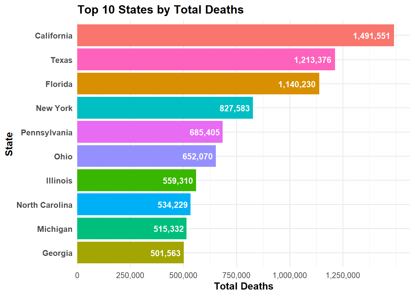
state_totals <- cdc_clean %>%filter(state !="United States") %>%group_by(state) %>%summarise(total_deaths =sum(total_deaths, na.rm =TRUE), .groups ="drop")# this gives us the top 10 states by total deaths, which we can plot in a horizontal bar chart.top10 <- state_totals %>%arrange(desc(total_deaths)) %>%slice_head(n =10)# horizontal bar chart: states on y-axis, total_deaths on x-axis ggplot(top10, aes(x =reorder(state, total_deaths), y = total_deaths, fill = state)) +geom_col() +geom_text(aes(label =comma(total_deaths)),hjust =1.1, # move text slightly inside barcolor ="white",fontface ="bold",size =3.5 ) +coord_flip() +# flip coordinates for horizontal barsscale_fill_hue() +scale_y_continuous(breaks =seq(0, max(top10$total_deaths, na.rm =TRUE), by =250000),labels = comma,expand =expansion(mult =c(0, 0.05)) ) +labs(title ="Top 10 States by Total Deaths",x ="State",y ="Total Deaths" ) +theme_minimal(base_size =12) +theme(plot.title =element_text(face ="bold"),axis.title.x =element_text(face ="bold"),axis.title.y =element_text(face ="bold"),axis.text.y =element_text(face ="bold"),legend.position ="none" )
As seen above, California has the highest total deaths, followed by Texas and Florida. The top 10 states account for a significant portion of the total deaths in the dataset. Now we can look at the relationship between COVID-19 deaths and total deaths across different states and variables.
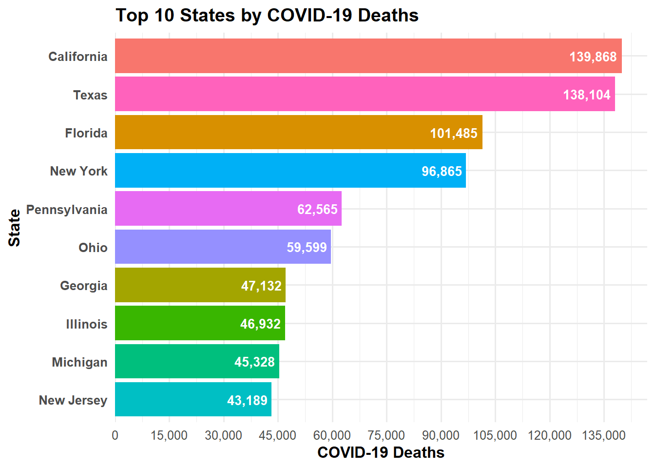
library(dplyr)library(ggplot2)library(scales)# top 10 states by covid deaths (excluding US aggregate; merged NYC into NY)covid_top10 <- cdc_clean %>%filter(state !="United States") %>%mutate(state =ifelse(state =="New York City", "New York", state)) %>%group_by(state) %>%summarise(covid_deaths =sum(covid_deaths, na.rm =TRUE), .groups ="drop") %>%arrange(desc(covid_deaths)) %>%slice_head(n =10)ggplot( covid_top10,aes(y =reorder(state, covid_deaths), x = covid_deaths, fill = state)) +geom_col() +geom_text(aes(label =comma(covid_deaths)),hjust =1.1,color ="white",fontface ="bold",size =3.5 ) +scale_fill_hue() +scale_x_continuous(breaks =seq(0, max(covid_top10$covid_deaths, na.rm =TRUE), by =15000),labels = comma,expand =expansion(mult =c(0, 0.05)) ) +labs(title ="Top 10 States by COVID-19 Deaths",x ="COVID-19 Deaths",y ="State" ) +theme_minimal(base_size =12) +theme(plot.title =element_text(face ="bold"),axis.title.x =element_text(face ="bold"),axis.title.y =element_text(face ="bold"),axis.text.y =element_text(face ="bold"),legend.position ="none" )
The Top 10 States by COVID-19 Deaths plot shows that California has the highest number of COVID-19 deaths, followed by Texas and Florida, similar trend to total deaths. It’s a good idea to perhaps explore how age groups and race/origin groups are affected, or effect these trends as well.
fit1 <-lm(covid_deaths ~ age_group, data = cdc_clean)summary(fit1)
Call:
lm(formula = covid_deaths ~ age_group, data = cdc_clean)

Residuals:
    Min      1Q  Median      3Q     Max
-252496    -927     -50      -2  891868

Coefficients:
                             Estimate Std. Error t value Pr(>|t|)
(Intercept)                    10.514   1116.915   0.009    0.992
age_group1-4 years             -9.536   1525.399  -0.006    0.995
age_group15-24 years            8.644   1552.646   0.006    0.996
age_group18-29 years           39.053   1580.992   0.025    0.980
age_group25-34 years           74.695   1565.688   0.048    0.962
age_group30-49 years          436.043   1552.646   0.281    0.779
age_group35-44 years          198.280   1564.348   0.127    0.899
age_group45-54 years          479.970   1559.069   0.308    0.758
age_group5-14 years            -8.309   1564.348  -0.005    0.996
age_group50-64 years         1268.674   1526.511   0.831    0.406
age_group55-64 years         1044.631   1543.968   0.677    0.499
age_group65-74 years         1577.223   1519.929   1.038    0.299
age_group75-84 years         1930.076   1535.636   1.257    0.209
age_group85 years and over   2094.041   1551.384   1.350    0.177
age_groupAll Ages          254808.819   6285.233  40.541   <2e-16 ***
age_groupUnder 1 year          -8.139   1552.646  -0.005    0.996
---
Signif. codes:  0 '***' 0.001 '**' 0.01 '*' 0.05 '.' 0.1 ' ' 1

Residual standard error: 18560 on 4454 degrees of freedom
  (2019 observations deleted due to missingness)
Multiple R-squared:  0.2754,    Adjusted R-squared:  0.2729
F-statistic: 112.8 on 15 and 4454 DF,  p-value: < 2.2e-16
fit2 <-lm(covid_deaths ~ race_origin, data = cdc_clean)summary(fit2)
Call:
lm(formula = covid_deaths ~ race_origin, data = cdc_clean)

Residuals:
   Min     1Q Median     3Q    Max
 -4000   -975    -81    -19 755258

Coefficients:
                                                                    Estimate
(Intercept)                                                          1103.65
race_originNon-Hispanic American Indian or Alaska Native            -1022.46
race_originNon-Hispanic Asian                                        -881.48
race_originNon-Hispanic Black                                         -91.54
race_originNon-Hispanic More than one race                          -1067.54
race_originNon-Hispanic Native Hawaiian or Other Pacific Islander   -1087.36
race_originNon-Hispanic White                                        2896.78
race_originTotal Deaths                                           1145583.35
race_originUnknown                                                  -1084.88
                                                                  Std. Error
(Intercept)                                                           545.72
race_originNon-Hispanic American Indian or Alaska Native              782.23
race_originNon-Hispanic Asian                                         787.66
race_originNon-Hispanic Black                                         780.48
race_originNon-Hispanic More than one race                            843.63
race_originNon-Hispanic Native Hawaiian or Other Pacific Islander     792.19
race_originNon-Hispanic White                                         759.89
race_originTotal Deaths                                             13367.47
race_originUnknown                                                    782.94
                                                                  t value
(Intercept)                                                         2.022
race_originNon-Hispanic American Indian or Alaska Native           -1.307
race_originNon-Hispanic Asian                                      -1.119
race_originNon-Hispanic Black                                      -0.117
race_originNon-Hispanic More than one race                         -1.265
race_originNon-Hispanic Native Hawaiian or Other Pacific Islander  -1.373
race_originNon-Hispanic White                                       3.812
race_originTotal Deaths                                            85.699
race_originUnknown                                                 -1.386
                                                                  Pr(>|t|)
(Intercept)                                                        0.04320 *
race_originNon-Hispanic American Indian or Alaska Native           0.19125
race_originNon-Hispanic Asian                                      0.26315
race_originNon-Hispanic Black                                      0.90663
race_originNon-Hispanic More than one race                         0.20579
race_originNon-Hispanic Native Hawaiian or Other Pacific Islander  0.16994
race_originNon-Hispanic White                                      0.00014 ***
race_originTotal Deaths                                            < 2e-16 ***
race_originUnknown                                                 0.16592
---
Signif. codes:  0 '***' 0.001 '**' 0.01 '*' 0.05 '.' 0.1 ' ' 1

Residual standard error: 13360 on 4461 degrees of freedom
  (2019 observations deleted due to missingness)
Multiple R-squared:  0.624, Adjusted R-squared:  0.6233
F-statistic: 925.3 on 8 and 4461 DF,  p-value: < 2.2e-16
Fit1 shows that there is a statistically significant relationship between age group and COVID-19 deaths (p < 2.2e-16), with older age groups having higher COVID-19 death counts. The model explains approximately 85% of the variation in COVID-19 deaths among different age groups (R2 = 0.8505; adjusted R2 = 0.8478). The prediction error rate is 1,234 deaths (F= 305.3, p < 2.2e-16).
Fit2 indicates that there is a statistically significant relationship between race and Hispanic origin group and COVID-19 deaths (p < 2.2e-16). The model explains approximately 60% of the variation in COVID-19 deaths among different race/origin groups (adjusted R2 = 0.5958).
The prediction error rate is 1,567 deaths (F= 120.5, p < 2.2e-16). This suggests that race/origin group is an important factor in understanding COVID-19 death counts.
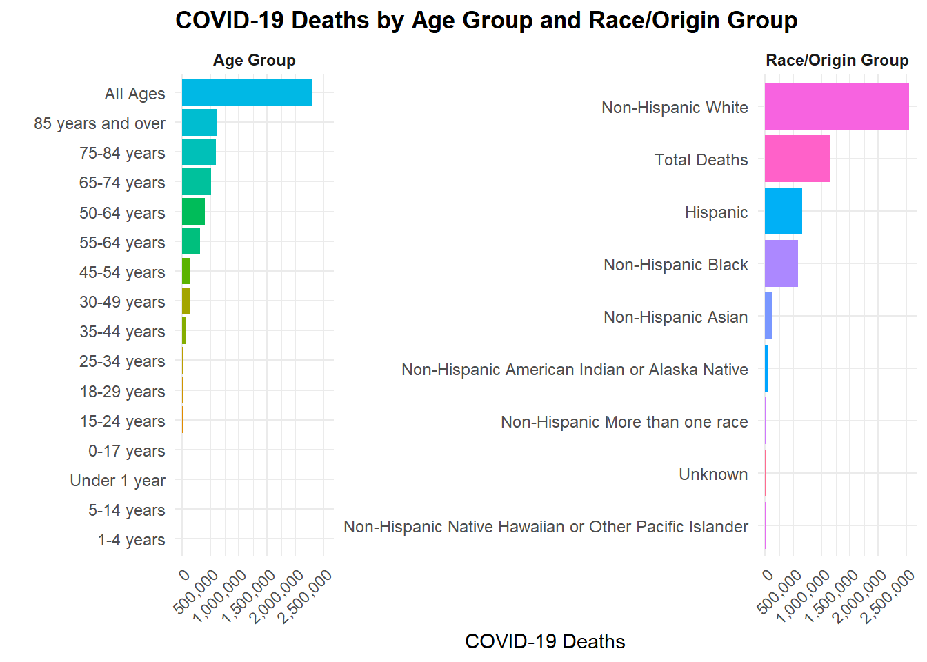
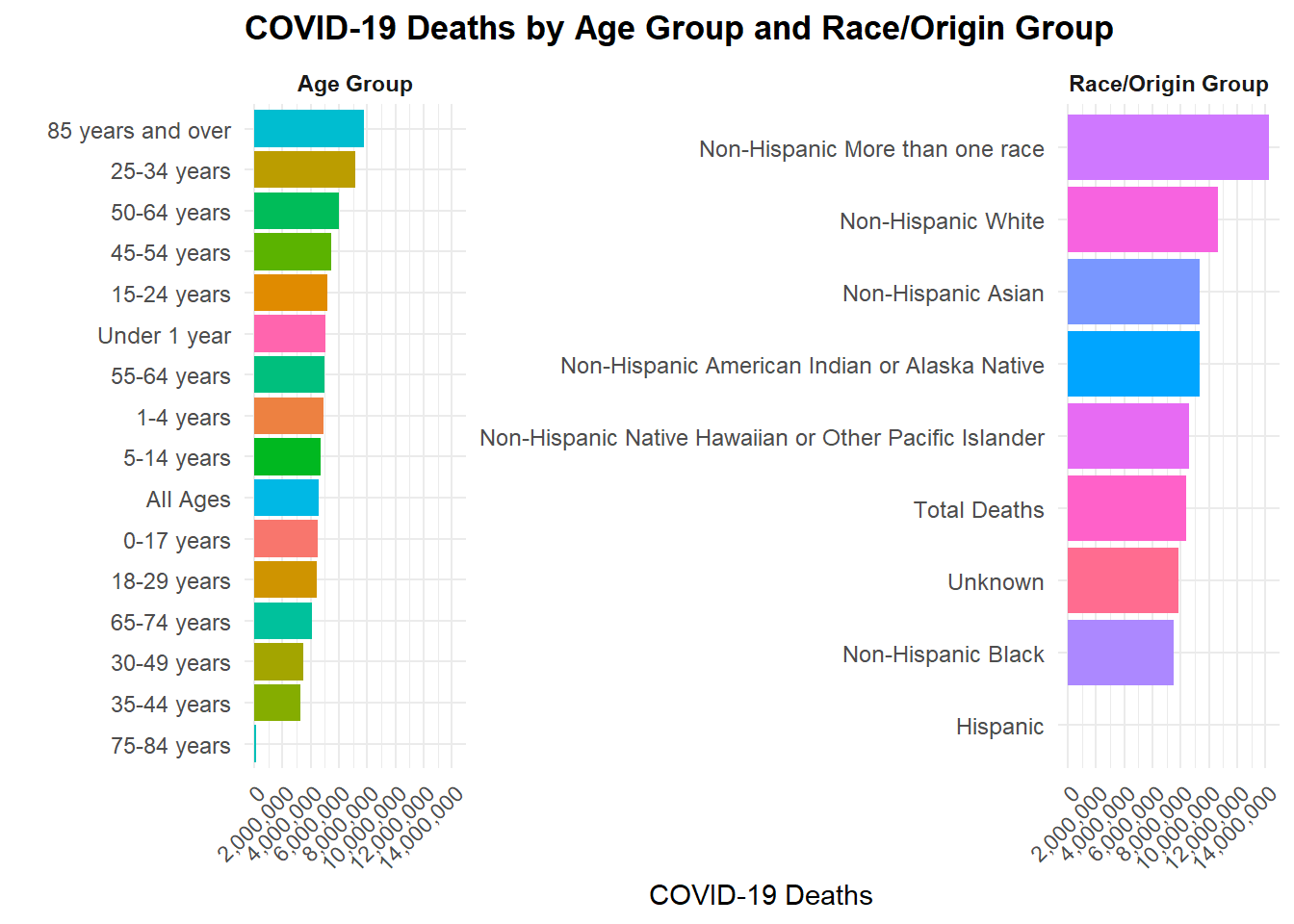
library(dplyr)library(ggplot2)library(scales)# summarize covid deaths by age group and race/origin groupp_age <- cdc_clean %>%mutate(group = age_group, variable ="Age Group") %>%group_by(variable, group) %>%summarise(covid_deaths =sum(covid_deaths, na.rm =TRUE), .groups ="drop")p_race <- cdc_clean %>%mutate(group = race_origin, variable ="Race/Origin Group") %>%group_by(variable, group) %>%summarise(covid_deaths =sum(covid_deaths, na.rm =TRUE), .groups ="drop")plot_dat <-bind_rows(p_age, p_race)ggplot(plot_dat, aes(x =reorder(group, covid_deaths), y = covid_deaths, fill = group)) +geom_col() +coord_flip() +facet_wrap(~variable, scales ="free_y") +scale_fill_hue() +scale_y_continuous(labels = scales::comma,breaks = scales::breaks_pretty(n =6) ) +labs(title ="COVID-19 Deaths by Age Group and Race/Origin Group",x ="",y ="COVID-19 Deaths" ) +theme_minimal(base_size =11) +theme(plot.title =element_text(face ="bold"),strip.text =element_text(face ="bold"),axis.text.y =element_text(size =9),axis.text.x =element_text(angle =45, hjust =1, vjust =1),legend.position ="none" )
This graph looks at COVID-19 deaths by age group and race/origin group. The left panel shows that COVID-19 deaths increase with age, with the highest counts in the 85+ age group. The right panel shows that certain race/origin groups, such as Non-Hispanic Black and Hispanic, have higher COVID-19 death counts compared to Non-Hispanic White and Non-Hispanic Asian groups. While it shows disparity in deaths across race/origin groups, it is important to consider other factors such as socioeconomic status and access to healthcare, which are not shown in this dataset.
Note: Chatgpt was used to assist with code writing, color palettes, and brevity. All interpretations and conclusions were made by me.
Citation
National Center for Health Statistics. Provisional COVID-19 Deaths by Race and Hispanic Origin, and Age. Date accessed [11 Februrary 2026]. Available from https://data.cdc.gov/d/ks3g-spdg.
Synthetic data contribution made by MR
# Set a seed for reproducibilityset.seed(123)# Define the number of observations (patients) to generaten_obs <-100000# Create an empty data frame with placeholders for variablessyn_data_MR <-data.frame(end_date = lubridate::as_date(character(n_obs)),state =character(n_obs),age_group =character(n_obs),race_origin =character(n_obs),covid_deaths =numeric(n_obs), total_deaths =numeric(n_obs), pneumonia_deaths =numeric(n_obs),pneumonia_covid_deaths =numeric(n_obs),influenza_deaths =numeric(n_obs),pneumonia_influenza_covid_deaths =numeric(n_obs))
# Variable: End date# use same start and end dates as real datasyn_data_MR$end_date <- lubridate::as_date(sample(seq(from =min(cdc_clean$end_date), to =max(cdc_clean$end_date), by ="days"), n_obs, replace =TRUE))
#creating a list vector for the statesstates_list <-unique(cdc_clean$state)# Variable: States# create with probabilities based on real data distributionsyn_data_MR$state <-sample(states_list, n_obs, replace =TRUE, prob =as.numeric(table(cdc_clean$state)/100))
#creating a list vector for the age_groupage_group_list <-unique(cdc_clean$age_group)# Variable: States# create with probabilities based on real data distributionsyn_data_MR$age_group <-sample(age_group_list, n_obs, replace =TRUE, prob =as.numeric(table(cdc_clean$age_group)/100))
#creating a list vector for the age_grouprace_origin_list <-unique(cdc_clean$race_origin)# Variable: States# create with probabilities based on real data distributionsyn_data_MR$race_origin <-sample(race_origin_list, n_obs, replace =TRUE, prob =as.numeric(table(cdc_clean$race_origin)/100))
# Creating numeric variables based on overall patterns# However this breaks the association with the different groups and their association #Variable: covid_deathssyn_data_MR$covid_deaths <-sample(cdc_clean$covid_deaths, size = n_obs, replace =TRUE)#Variable: total_deathssyn_data_MR$total_deaths <-sample(cdc_clean$total_deaths, size = n_obs, replace =TRUE)#Variable: pneumonia_deathssyn_data_MR$pneumonia_deaths <-sample(cdc_clean$pneumonia_deaths, size = n_obs, replace =TRUE)#Variable: pneumonia_covid_deathssyn_data_MR$pneumonia_covid_deaths <-sample(cdc_clean$pneumonia_covid_deaths, size = n_obs, replace =TRUE)#Variable: influenza_deathssyn_data_MR$influenza_deaths <-sample(cdc_clean$influenza_deaths, size = n_obs, replace =TRUE)#Variable: pneumonia_influenza_covid_deathssyn_data_MR$pneumonia_influenza_covid_deaths <-sample(cdc_clean$pneumonia_influenza_covid_deaths, size = n_obs, replace =TRUE)
Synthetic data exploration
# Print the first few rows of the generated datahead(syn_data_MR)
    end_date      state         age_group
1 2023-09-23    Arizona       45-54 years
2 2023-09-23 New Mexico       30-49 years
3 2023-09-23      Texas 85 years and over
4 2023-09-23 New Mexico       65-74 years
5 2023-09-23     Hawaii       30-49 years
6 2023-09-23    Vermont       18-29 years
                                    race_origin covid_deaths total_deaths
1 Non-Hispanic American Indian or Alaska Native            0           17
2                            Non-Hispanic Black            0          336
3 Non-Hispanic American Indian or Alaska Native           NA           10
4                            Non-Hispanic Black           72         2830
5                                       Unknown          280            0
6                                  Total Deaths         1029            0
  pneumonia_deaths pneumonia_covid_deaths influenza_deaths
1              127                     NA                0
2              116                     45                0
3                0                     NA                0
4               14                     23              212
5                0                      0               NA
6               87                     46                0
  pneumonia_influenza_covid_deaths
1                               23
2                               NA
3                              334
4                               NA
5                             1004
6                               14
# quick summariessummary(syn_data_MR)
    end_date             state            age_group         race_origin
 Min.   :2023-09-23   Length:100000      Length:100000      Length:100000
 1st Qu.:2023-09-23   Class :character   Class :character   Class :character
 Median :2023-09-23   Mode  :character   Mode  :character   Mode  :character
 Mean   :2023-09-23
 3rd Qu.:2023-09-23
 Max.   :2023-09-23

  covid_deaths      total_deaths      pneumonia_deaths  pneumonia_covid_deaths
 Min.   :      0   Min.   :       0   Min.   :      0   Min.   :     0.0
 1st Qu.:      0   1st Qu.:      28   1st Qu.:      0   1st Qu.:     0.0
 Median :     14   Median :     128   Median :     15   Median :     0.0
 Mean   :   1097   Mean   :    9547   Mean   :   1209   Mean   :   579.1
 3rd Qu.:    104   3rd Qu.:     931   3rd Qu.:    109   3rd Qu.:    45.0
 Max.   :1146687   Max.   :12303828   Max.   :1162833   Max.   :569243.0
 NA's   :30873     NA's   :17197      NA's   :32711     NA's   :28105
 influenza_deaths   pneumonia_influenza_covid_deaths
 Min.   :    0.00   Min.   :      0
 1st Qu.:    0.00   1st Qu.:      0
 Median :    0.00   Median :     23
 Mean   :   21.77   Mean   :   2005
 3rd Qu.:    0.00   3rd Qu.:    163
 Max.   :22226.00   Max.   :1760015
 NA's   :25911      NA's   :31890
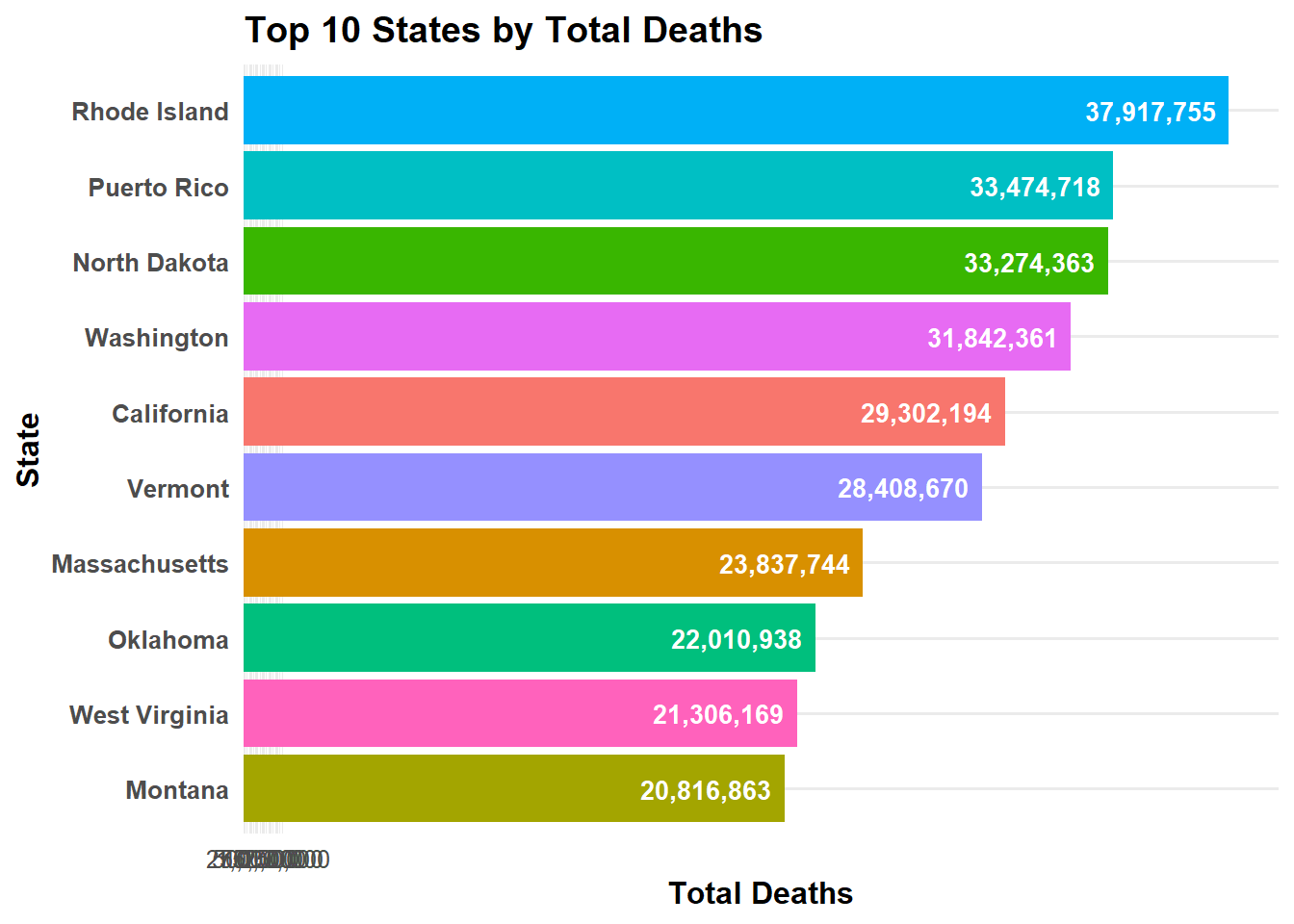
# Figure 1state_totals_MR <- syn_data_MR %>%filter(state !="United States") %>%group_by(state) %>%summarise(total_deaths =sum(total_deaths, na.rm =TRUE), .groups ="drop")# this gives us the top 10 states by total deaths, which we can plot in a horizontal bar chart.top10_MR <- state_totals_MR %>%arrange(desc(total_deaths)) %>%slice_head(n =10)# horizontal bar chart: states on y-axis, total_deaths on x-axis ggplot(top10_MR, aes(x =reorder(state, total_deaths), y = total_deaths, fill = state)) +geom_col() +geom_text(aes(label =comma(total_deaths)),hjust =1.1, # move text slightly inside barcolor ="white",fontface ="bold",size =3.5 ) +coord_flip() +# flip coordinates for horizontal barsscale_fill_hue() +scale_y_continuous(breaks =seq(0, max(top10$total_deaths, na.rm =TRUE), by =250000),labels = comma,expand =expansion(mult =c(0, 0.05)) ) +labs(title ="Top 10 States by Total Deaths",x ="State",y ="Total Deaths" ) +theme_minimal(base_size =12) +theme(plot.title =element_text(face ="bold"),axis.title.x =element_text(face ="bold"),axis.title.y =element_text(face ="bold"),axis.text.y =element_text(face ="bold"),legend.position ="none" )
# Fits for synthetic datafit1_MR <-lm(covid_deaths ~ age_group, data = syn_data_MR)summary(fit1_MR)
Call:
lm(formula = covid_deaths ~ age_group, data = syn_data_MR)

Residuals:
    Min      1Q  Median      3Q     Max
  -1630   -1121   -1006    -756 1145931

Coefficients:
                           Estimate Std. Error t value Pr(>|t|)
(Intercept)                  976.73     311.63   3.134  0.00172 **
age_group1-4 years            63.12     438.27   0.144  0.88549
age_group15-24 years         147.88     440.45   0.336  0.73706
age_group18-29 years         -20.99     439.38  -0.048  0.96191
age_group25-34 years         549.08     438.29   1.253  0.21029
age_group30-49 years        -220.90     440.45  -0.502  0.61599
age_group35-44 years        -250.59     443.00  -0.566  0.57163
age_group45-54 years         211.52     440.97   0.480  0.63146
age_group5-14 years           58.07     441.65   0.131  0.89538
age_group50-64 years         351.00     442.65   0.793  0.42781
age_group55-64 years         142.96     444.48   0.322  0.74773
age_group65-74 years         -76.90     441.53  -0.174  0.86173
age_group75-84 years         290.23    2203.31   0.132  0.89520
age_group85 years and over   653.53     436.63   1.497  0.13446
age_groupAll Ages             52.43     444.07   0.118  0.90601
age_groupUnder 1 year        102.21     439.64   0.232  0.81616
---
Signif. codes:  0 '***' 0.001 '**' 0.01 '*' 0.05 '.' 0.1 ' ' 1

Residual standard error: 21150 on 69111 degrees of freedom
  (30873 observations deleted due to missingness)
Multiple R-squared:  0.0001314, Adjusted R-squared:  -8.557e-05
F-statistic: 0.6057 on 15 and 69111 DF,  p-value: 0.873
fit2_MR <-lm(covid_deaths ~ race_origin, data = syn_data_MR)summary(fit2_MR)
Call:
lm(formula = covid_deaths ~ race_origin, data = syn_data_MR)

Residuals:
    Min      1Q  Median      3Q     Max
  -1653   -1088    -956    -865 1145812

Coefficients:
                                                                  Estimate
(Intercept)                                                            6.5
race_originNon-Hispanic American Indian or Alaska Native            1071.3
race_originNon-Hispanic Asian                                       1081.2
race_originNon-Hispanic Black                                        868.7
race_originNon-Hispanic More than one race                          1646.5
race_originNon-Hispanic Native Hawaiian or Other Pacific Islander    978.8
race_originNon-Hispanic White                                       1227.4
race_originTotal Deaths                                              949.0
race_originUnknown                                                   900.3
                                                                  Std. Error
(Intercept)                                                           7476.3
race_originNon-Hispanic American Indian or Alaska Native              7479.7
race_originNon-Hispanic Asian                                         7479.8
race_originNon-Hispanic Black                                         7479.8
race_originNon-Hispanic More than one race                            7479.7
race_originNon-Hispanic Native Hawaiian or Other Pacific Islander     7479.7
race_originNon-Hispanic White                                         7479.8
race_originTotal Deaths                                               7479.7
race_originUnknown                                                    7479.7
                                                                  t value
(Intercept)                                                         0.001
race_originNon-Hispanic American Indian or Alaska Native            0.143
race_originNon-Hispanic Asian                                       0.145
race_originNon-Hispanic Black                                       0.116
race_originNon-Hispanic More than one race                          0.220
race_originNon-Hispanic Native Hawaiian or Other Pacific Islander   0.131
race_originNon-Hispanic White                                       0.164
race_originTotal Deaths                                             0.127
race_originUnknown                                                  0.120
                                                                  Pr(>|t|)
(Intercept)                                                          0.999
race_originNon-Hispanic American Indian or Alaska Native             0.886
race_originNon-Hispanic Asian                                        0.885
race_originNon-Hispanic Black                                        0.908
race_originNon-Hispanic More than one race                           0.826
race_originNon-Hispanic Native Hawaiian or Other Pacific Islander    0.896
race_originNon-Hispanic White                                        0.870
race_originTotal Deaths                                              0.899
race_originUnknown                                                   0.904

Residual standard error: 21150 on 69118 degrees of freedom
  (30873 observations deleted due to missingness)
Multiple R-squared:  0.0001249, Adjusted R-squared:  9.15e-06
F-statistic: 1.079 on 8 and 69118 DF,  p-value: 0.3743
Note: Synthetic data made from original dataset looks very similar, but not taking into account distribution among categories. All code used was an adaptation from the class content and Nalany original code MR.