This data analysis was done using the Provisional COVID-19 Deaths by Race and Hispanic Origin, and Age dataset provided by the NCHS/DVS, which contains data on deaths involving COVID-19, pneumonia, and influenza, categorized by race/age/jurisdiction.
There are 13 columns listed:
Date as of - date of analysis
Start date - first date of data period
End date - last date of data period
State - jurisdiction of occurrence
Age group - age group
Race and Hispanic Origin Group - Race or Hispanic origin group
Pneumonia, Influenza, or COVID-19 deaths - deaths with any of aforementioned codes.
Footnote- suppressed counts (1-9)
Package loading and install
First we need to upload and/or install packages for cleaning our data
Show the code
# install packages if not already installed (run once in the console)# load required packages# tidyverse added for later steps with data processinglibrary("dslabs")library("tidyverse")
── Attaching core tidyverse packages ──────────────────────── tidyverse 2.0.0 ──
✔ dplyr     1.2.1     ✔ readr     2.2.0
✔ forcats   1.0.1     ✔ stringr   1.6.0
✔ ggplot2   4.0.3     ✔ tibble    3.3.1
✔ lubridate 1.9.5     ✔ tidyr     1.3.2
✔ purrr     1.2.2
── Conflicts ────────────────────────────────────────── tidyverse_conflicts() ──
✖ dplyr::filter() masks stats::filter()
✖ dplyr::lag()    masks stats::lag()
ℹ Use the conflicted package (<http://conflicted.r-lib.org/>) to force all conflicts to become errors
Show the code
library("readr")library("stringr")library("here")
here() starts at /Users/nalanyrichardson/Downloads/MADA/Portfolio
Show the code
library("janitor")
Attaching package: 'janitor'

The following objects are masked from 'package:stats':

    chisq.test, fisher.test
Show the code
# read in the datacdcdata <-read_csv(here("cdcdata-exercise", "Provisional_COVID-19_Deaths_by_Race_and_Hispanic_Origin,_and_Age_20260211.csv"))
Rows: 6489 Columns: 13
── Column specification ────────────────────────────────────────────────────────
Delimiter: ","
chr (7): Data as of, Start Date, End Date, State, Age group, Race and Hispan...
num (6): COVID-19 Deaths, Total Deaths, Pneumonia Deaths, Pneumonia and COVI...

ℹ Use `spec()` to retrieve the full column specification for this data.
ℹ Specify the column types or set `show_col_types = FALSE` to quiet this message.
Show dataset structure
Now we should take a look at what the data actually looks like.
Show the code
# get an overview of data structure# I prefer str() for checking out the data, but I also like glimpse() for very rote summaries where you can determine characteristics.We can run all of them and see what we get, and then just choose whatever we'd like.str(cdcdata)
spc_tbl_ [6,489 × 13] (S3: spec_tbl_df/tbl_df/tbl/data.frame)
 $ Data as of                              : chr [1:6489] "09/27/2023" "09/27/2023" "09/27/2023" "09/27/2023" ...
 $ Start Date                              : chr [1:6489] "01/01/2020" "01/01/2020" "01/01/2020" "01/01/2020" ...
 $ End Date                                : chr [1:6489] "09/23/2023" "09/23/2023" "09/23/2023" "09/23/2023" ...
 $ State                                   : chr [1:6489] "United States" "United States" "United States" "United States" ...
 $ Age group                               : chr [1:6489] "All Ages" "All Ages" "Under 1 year" "0-17 years" ...
 $ Race and Hispanic Origin Group          : chr [1:6489] "Total Deaths" "Non-Hispanic White" "Non-Hispanic White" "Non-Hispanic White" ...
 $ COVID-19 Deaths                         : num [1:6489] 1146687 759258 190 642 113 ...
 $ Total Deaths                            : num [1:6489] 12303828 9104563 28980 54364 6164 ...
 $ Pneumonia Deaths                        : num [1:6489] 1162833 805461 409 1218 278 ...
 $ Pneumonia and COVID-19 Deaths           : num [1:6489] 569243 362196 34 163 28 ...
 $ Influenza Deaths                        : num [1:6489] 22226 16132 24 248 84 ...
 $ Pneumonia, Influenza, or COVID-19 Deaths: num [1:6489] 1760015 1217336 588 1931 443 ...
 $ Footnote                                : chr [1:6489] NA NA NA NA ...
 - attr(*, "spec")=
  .. cols(
  ..   `Data as of` = col_character(),
  ..   `Start Date` = col_character(),
  ..   `End Date` = col_character(),
  ..   State = col_character(),
  ..   `Age group` = col_character(),
  ..   `Race and Hispanic Origin Group` = col_character(),
  ..   `COVID-19 Deaths` = col_number(),
  ..   `Total Deaths` = col_number(),
  ..   `Pneumonia Deaths` = col_number(),
  ..   `Pneumonia and COVID-19 Deaths` = col_number(),
  ..   `Influenza Deaths` = col_number(),
  ..   `Pneumonia, Influenza, or COVID-19 Deaths` = col_number(),
  ..   Footnote = col_character()
  .. )
 - attr(*, "problems")=<pointer: 0x76edf55c0>
library(dplyr)library(readr)# clean datacdc_clean <- cdcdata %>%# remove columns not needed for our analysisselect(-`Data as of`, -`Start Date`, -Footnote) %>%# rename columns-- I do this as the original dataset would require backticks for uppercase and spaced column names.rename(end_date =`End Date`,state = State,age_group =`Age group`,race_origin =`Race and Hispanic Origin Group`,covid_deaths =`COVID-19 Deaths`,total_deaths =`Total Deaths`,pneumonia_deaths =`Pneumonia Deaths`,pneumonia_covid_deaths =`Pneumonia and COVID-19 Deaths`,influenza_deaths =`Influenza Deaths`,pneumonia_influenza_covid_deaths =`Pneumonia, Influenza, or COVID-19 Deaths` ) %>%# standardize formats and clean spacing. `mdy()` converts the end_date column to a date format, while `str_squish()` and `str_trim()` remove extra spaces from the state. I noticed that some state values were returning as `NA` because of extra spaces. So look out for that!mutate(end_date =mdy(end_date),state =str_squish(str_trim(state)),age_group =str_squish(str_trim(age_group)),race_origin =str_squish(str_trim(race_origin)) )# also saw that NYC was separated from New York, so I combined those two together to avoid confusion and make sure all data from New York is in one place.cdc_clean <- cdc_clean %>%mutate(state =ifelse(state %in%c("New York", "New York City"), "New York", state))# now we can double check that names are correct and data is in the correct format.names(cdc_clean)
We can now start to analyze the data and make some plots. For example, we can look at the relationship between COVID-19 deaths and total deaths across different age groups or states.
We can also explore how pneumonia deaths relate to COVID-19 deaths, or how influenza deaths compare across different race and Hispanic origin groups.
Show the code
library(dplyr)library(ggplot2)library(scales)
Attaching package: 'scales'
The following object is masked from 'package:purrr':

    discard
The following object is masked from 'package:readr':

    col_factor
Show the code
state_totals <- cdc_clean %>%filter(state !="United States") %>%group_by(state) %>%summarise(total_deaths =sum(total_deaths, na.rm =TRUE), .groups ="drop")# this gives us the top 10 states by total deaths, which we can plot in a horizontal bar chart.top10 <- state_totals %>%arrange(desc(total_deaths)) %>%slice_head(n =10)# horizontal bar chart: states on y-axis, total_deaths on x-axis ggplot(top10, aes(x =reorder(state, total_deaths), y = total_deaths, fill = state)) +geom_col() +geom_text(aes(label =comma(total_deaths)),hjust =1.1, # move text slightly inside barcolor ="white",fontface ="bold",size =3.5 ) +coord_flip() +# flip coordinates for horizontal barsscale_fill_hue() +scale_y_continuous(breaks =seq(0, max(top10$total_deaths, na.rm =TRUE), by =250000),labels = comma,expand =expansion(mult =c(0, 0.05)) ) +labs(title ="Top 10 States by Total Deaths",x ="State",y ="Total Deaths" ) +theme_minimal(base_size =12) +theme(plot.title =element_text(face ="bold"),axis.title.x =element_text(face ="bold"),axis.title.y =element_text(face ="bold"),axis.text.y =element_text(face ="bold"),legend.position ="none" )
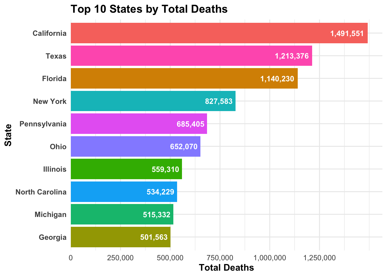
As seen above, California has the highest total deaths, followed by Texas and Florida. The top 10 states account for a significant portion of the total deaths in the dataset. Now we can look at the relationship between COVID-19 deaths and total deaths across different states and variables.
Show the code
library(dplyr)library(ggplot2)library(scales)# top 10 states by covid deaths (excluding US aggregate; merged NYC into NY)covid_top10 <- cdc_clean %>%filter(state !="United States") %>%mutate(state =ifelse(state =="New York City", "New York", state)) %>%group_by(state) %>%summarise(covid_deaths =sum(covid_deaths, na.rm =TRUE), .groups ="drop") %>%arrange(desc(covid_deaths)) %>%slice_head(n =10)ggplot( covid_top10,aes(y =reorder(state, covid_deaths), x = covid_deaths, fill = state)) +geom_col() +geom_text(aes(label =comma(covid_deaths)),hjust =1.1,color ="white",fontface ="bold",size =3.5 ) +scale_fill_hue() +scale_x_continuous(breaks =seq(0, max(covid_top10$covid_deaths, na.rm =TRUE), by =15000),labels = comma,expand =expansion(mult =c(0, 0.05)) ) +labs(title ="Top 10 States by COVID-19 Deaths",x ="COVID-19 Deaths",y ="State" ) +theme_minimal(base_size =12) +theme(plot.title =element_text(face ="bold"),axis.title.x =element_text(face ="bold"),axis.title.y =element_text(face ="bold"),axis.text.y =element_text(face ="bold"),legend.position ="none" )
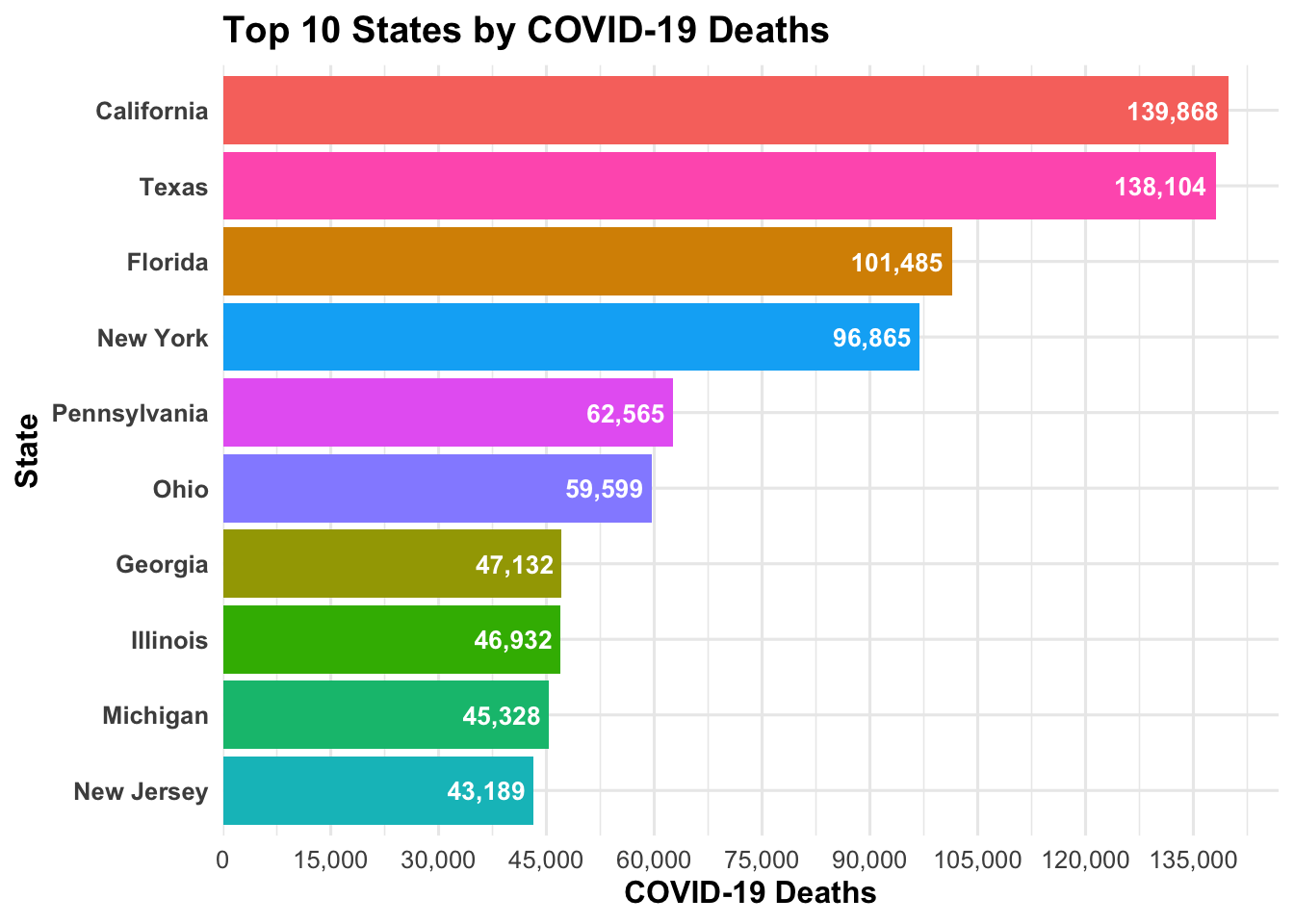
The Top 10 States by COVID-19 Deaths plot shows that California has the highest number of COVID-19 deaths, followed by Texas and Florida, similar trend to total deaths. It’s a good idea to perhaps explore how age groups and race/origin groups are affected, or effect these trends as well.
Show the code
fit1 <-lm(covid_deaths ~ age_group, data = cdc_clean)summary(fit1)
Call:
lm(formula = covid_deaths ~ age_group, data = cdc_clean)

Residuals:
    Min      1Q  Median      3Q     Max
-252496    -927     -50      -2  891868

Coefficients:
                             Estimate Std. Error t value Pr(>|t|)
(Intercept)                    10.514   1116.915   0.009    0.992
age_group1-4 years             -9.536   1525.399  -0.006    0.995
age_group15-24 years            8.644   1552.646   0.006    0.996
age_group18-29 years           39.053   1580.992   0.025    0.980
age_group25-34 years           74.695   1565.688   0.048    0.962
age_group30-49 years          436.043   1552.646   0.281    0.779
age_group35-44 years          198.280   1564.348   0.127    0.899
age_group45-54 years          479.970   1559.069   0.308    0.758
age_group5-14 years            -8.309   1564.348  -0.005    0.996
age_group50-64 years         1268.674   1526.511   0.831    0.406
age_group55-64 years         1044.631   1543.968   0.677    0.499
age_group65-74 years         1577.223   1519.929   1.038    0.299
age_group75-84 years         1930.076   1535.636   1.257    0.209
age_group85 years and over   2094.041   1551.384   1.350    0.177
age_groupAll Ages          254808.819   6285.233  40.541   <2e-16 ***
age_groupUnder 1 year          -8.139   1552.646  -0.005    0.996
---
Signif. codes:  0 '***' 0.001 '**' 0.01 '*' 0.05 '.' 0.1 ' ' 1

Residual standard error: 18560 on 4454 degrees of freedom
  (2019 observations deleted due to missingness)
Multiple R-squared:  0.2754,    Adjusted R-squared:  0.2729
F-statistic: 112.8 on 15 and 4454 DF,  p-value: < 2.2e-16
Show the code
fit2 <-lm(covid_deaths ~ race_origin, data = cdc_clean)summary(fit2)
Call:
lm(formula = covid_deaths ~ race_origin, data = cdc_clean)

Residuals:
   Min     1Q Median     3Q    Max
 -4000   -975    -81    -19 755258

Coefficients:
                                                                    Estimate
(Intercept)                                                          1103.65
race_originNon-Hispanic American Indian or Alaska Native            -1022.46
race_originNon-Hispanic Asian                                        -881.48
race_originNon-Hispanic Black                                         -91.54
race_originNon-Hispanic More than one race                          -1067.54
race_originNon-Hispanic Native Hawaiian or Other Pacific Islander   -1087.36
race_originNon-Hispanic White                                        2896.78
race_originTotal Deaths                                           1145583.35
race_originUnknown                                                  -1084.88
                                                                  Std. Error
(Intercept)                                                           545.72
race_originNon-Hispanic American Indian or Alaska Native              782.23
race_originNon-Hispanic Asian                                         787.66
race_originNon-Hispanic Black                                         780.48
race_originNon-Hispanic More than one race                            843.63
race_originNon-Hispanic Native Hawaiian or Other Pacific Islander     792.19
race_originNon-Hispanic White                                         759.89
race_originTotal Deaths                                             13367.47
race_originUnknown                                                    782.94
                                                                  t value
(Intercept)                                                         2.022
race_originNon-Hispanic American Indian or Alaska Native           -1.307
race_originNon-Hispanic Asian                                      -1.119
race_originNon-Hispanic Black                                      -0.117
race_originNon-Hispanic More than one race                         -1.265
race_originNon-Hispanic Native Hawaiian or Other Pacific Islander  -1.373
race_originNon-Hispanic White                                       3.812
race_originTotal Deaths                                            85.699
race_originUnknown                                                 -1.386
                                                                  Pr(>|t|)
(Intercept)                                                        0.04320 *
race_originNon-Hispanic American Indian or Alaska Native           0.19125
race_originNon-Hispanic Asian                                      0.26315
race_originNon-Hispanic Black                                      0.90663
race_originNon-Hispanic More than one race                         0.20579
race_originNon-Hispanic Native Hawaiian or Other Pacific Islander  0.16994
race_originNon-Hispanic White                                      0.00014 ***
race_originTotal Deaths                                            < 2e-16 ***
race_originUnknown                                                 0.16592
---
Signif. codes:  0 '***' 0.001 '**' 0.01 '*' 0.05 '.' 0.1 ' ' 1

Residual standard error: 13360 on 4461 degrees of freedom
  (2019 observations deleted due to missingness)
Multiple R-squared:  0.624, Adjusted R-squared:  0.6233
F-statistic: 925.3 on 8 and 4461 DF,  p-value: < 2.2e-16
Fit1 shows that there is a statistically significant relationship between age group and COVID-19 deaths (p < 2.2e-16), with older age groups having higher COVID-19 death counts. The model explains approximately 85% of the variation in COVID-19 deaths among different age groups (R2 = 0.8505; adjusted R2 = 0.8478). The prediction error rate is 1,234 deaths (F= 305.3, p < 2.2e-16).
Fit2 indicates that there is a statistically significant relationship between race and Hispanic origin group and COVID-19 deaths (p < 2.2e-16). The model explains approximately 60% of the variation in COVID-19 deaths among different race/origin groups (adjusted R2 = 0.5958).
The prediction error rate is 1,567 deaths (F= 120.5, p < 2.2e-16). This suggests that race/origin group is an important factor in understanding COVID-19 death counts.
Show the code
library(dplyr)library(ggplot2)library(scales)# summarize covid deaths by age group and race/origin groupp_age <- cdc_clean %>%mutate(group = age_group, variable ="Age Group") %>%group_by(variable, group) %>%summarise(covid_deaths =sum(covid_deaths, na.rm =TRUE), .groups ="drop")p_race <- cdc_clean %>%mutate(group = race_origin, variable ="Race/Origin Group") %>%group_by(variable, group) %>%summarise(covid_deaths =sum(covid_deaths, na.rm =TRUE), .groups ="drop")plot_dat <-bind_rows(p_age, p_race)ggplot(plot_dat, aes(x =reorder(group, covid_deaths), y = covid_deaths, fill = group)) +geom_col() +coord_flip() +facet_wrap(~variable, scales ="free_y") +scale_fill_hue() +scale_y_continuous(labels = scales::comma,breaks = scales::breaks_pretty(n =6) ) +labs(title ="COVID-19 Deaths by Age Group and Race/Origin Group",x ="",y ="COVID-19 Deaths" ) +theme_minimal(base_size =11) +theme(plot.title =element_text(face ="bold"),strip.text =element_text(face ="bold"),axis.text.y =element_text(size =9),axis.text.x =element_text(angle =45, hjust =1, vjust =1),legend.position ="none" )
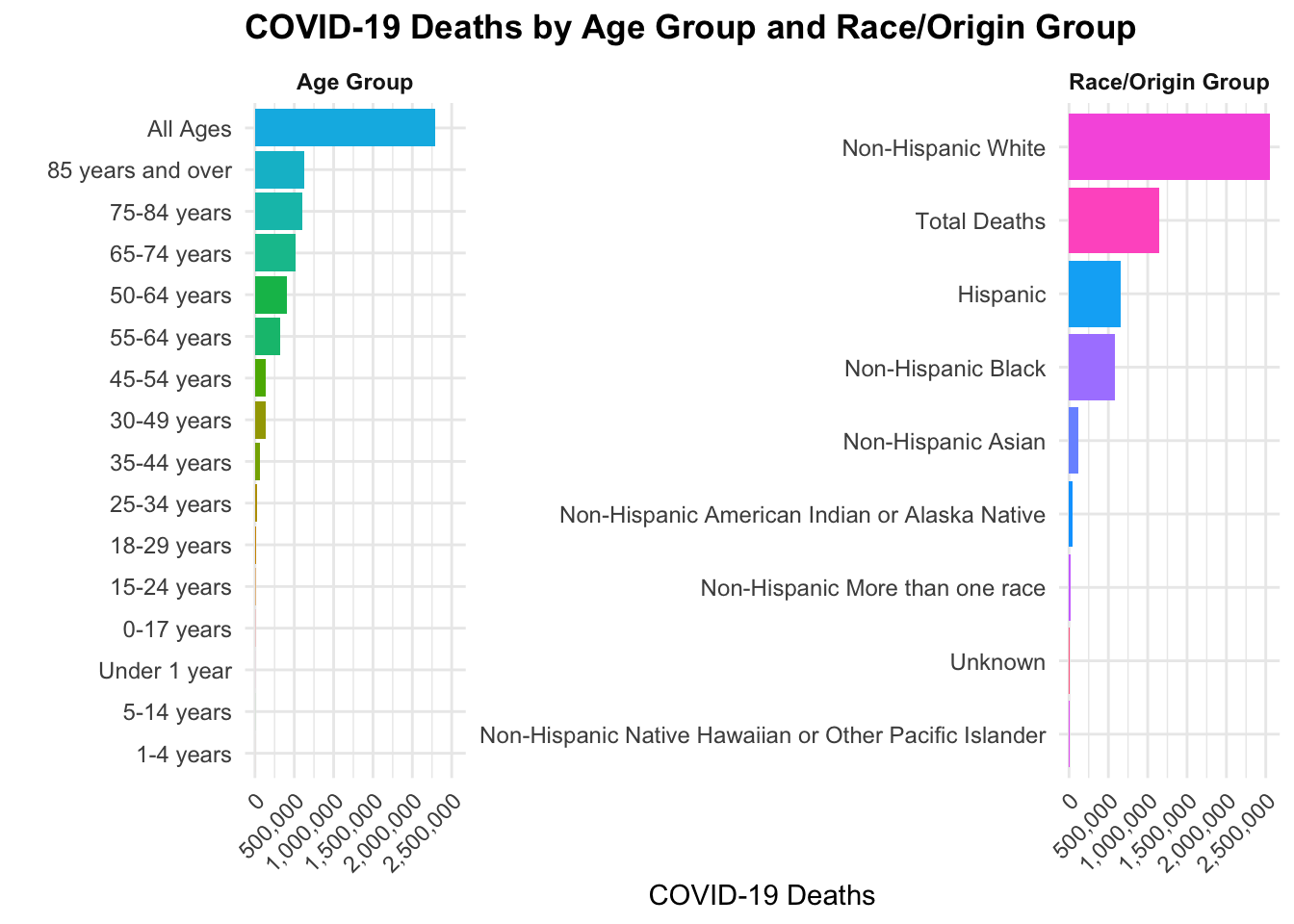
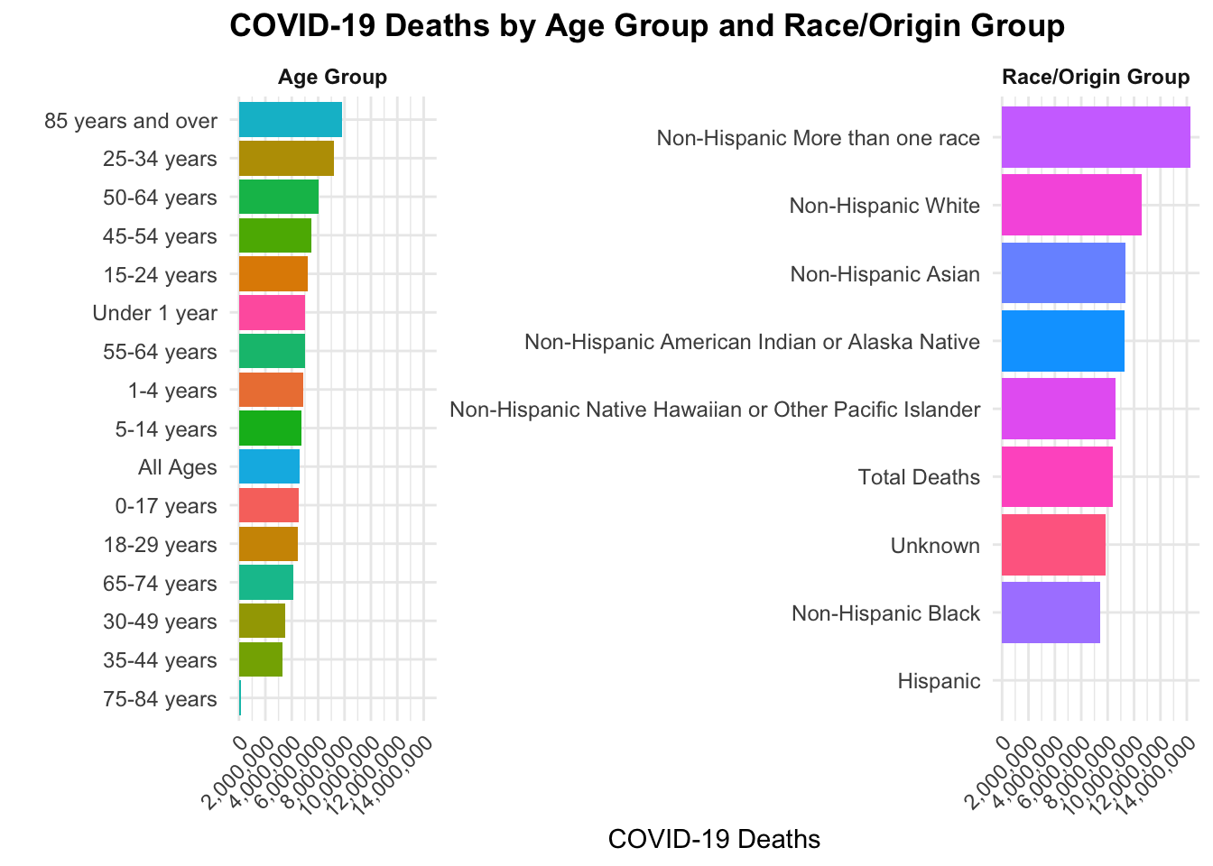
This graph looks at COVID-19 deaths by age group and race/origin group. The left panel shows that COVID-19 deaths increase with age, with the highest counts in the 85+ age group. The right panel shows that certain race/origin groups, such as Non-Hispanic Black and Hispanic, have higher COVID-19 death counts compared to Non-Hispanic White and Non-Hispanic Asian groups. While it shows disparity in deaths across race/origin groups, it is important to consider other factors such as socioeconomic status and access to healthcare, which are not shown in this dataset.
Note: Chatgpt was used to assist with code writing, color palettes, and brevity. All interpretations and conclusions were made by me.
Citation
National Center for Health Statistics. Provisional COVID-19 Deaths by Race and Hispanic Origin, and Age. Date accessed [11 Februrary 2026]. Available from https://data.cdc.gov/d/ks3g-spdg.
Synthetic data contribution made by MR
Show the code
# Set a seed for reproducibilityset.seed(123)# Define the number of observations (patients) to generaten_obs <-100000# Create an empty data frame with placeholders for variablessyn_data_MR <-data.frame(end_date = lubridate::as_date(character(n_obs)),state =character(n_obs),age_group =character(n_obs),race_origin =character(n_obs),covid_deaths =numeric(n_obs), total_deaths =numeric(n_obs), pneumonia_deaths =numeric(n_obs),pneumonia_covid_deaths =numeric(n_obs),influenza_deaths =numeric(n_obs),pneumonia_influenza_covid_deaths =numeric(n_obs))
Show the code
# Variable: End date# use same start and end dates as real datasyn_data_MR$end_date <- lubridate::as_date(sample(seq(from =min(cdc_clean$end_date), to =max(cdc_clean$end_date), by ="days"), n_obs, replace =TRUE))
Show the code
#creating a list vector for the statesstates_list <-unique(cdc_clean$state)# Variable: States# create with probabilities based on real data distributionsyn_data_MR$state <-sample(states_list, n_obs, replace =TRUE, prob =as.numeric(table(cdc_clean$state)/100))
Show the code
#creating a list vector for the age_groupage_group_list <-unique(cdc_clean$age_group)# Variable: States# create with probabilities based on real data distributionsyn_data_MR$age_group <-sample(age_group_list, n_obs, replace =TRUE, prob =as.numeric(table(cdc_clean$age_group)/100))
Show the code
#creating a list vector for the age_grouprace_origin_list <-unique(cdc_clean$race_origin)# Variable: States# create with probabilities based on real data distributionsyn_data_MR$race_origin <-sample(race_origin_list, n_obs, replace =TRUE, prob =as.numeric(table(cdc_clean$race_origin)/100))
Show the code
# Creating numeric variables based on overall patterns# However this breaks the association with the different groups and their association #Variable: covid_deathssyn_data_MR$covid_deaths <-sample(cdc_clean$covid_deaths, size = n_obs, replace =TRUE)#Variable: total_deathssyn_data_MR$total_deaths <-sample(cdc_clean$total_deaths, size = n_obs, replace =TRUE)#Variable: pneumonia_deathssyn_data_MR$pneumonia_deaths <-sample(cdc_clean$pneumonia_deaths, size = n_obs, replace =TRUE)#Variable: pneumonia_covid_deathssyn_data_MR$pneumonia_covid_deaths <-sample(cdc_clean$pneumonia_covid_deaths, size = n_obs, replace =TRUE)#Variable: influenza_deathssyn_data_MR$influenza_deaths <-sample(cdc_clean$influenza_deaths, size = n_obs, replace =TRUE)#Variable: pneumonia_influenza_covid_deathssyn_data_MR$pneumonia_influenza_covid_deaths <-sample(cdc_clean$pneumonia_influenza_covid_deaths, size = n_obs, replace =TRUE)
Synthetic data exploration
Show the code
# Print the first few rows of the generated datahead(syn_data_MR)
    end_date      state         age_group
1 2023-09-23    Arizona       45-54 years
2 2023-09-23 New Mexico       30-49 years
3 2023-09-23      Texas 85 years and over
4 2023-09-23 New Mexico       65-74 years
5 2023-09-23     Hawaii       30-49 years
6 2023-09-23    Vermont       18-29 years
                                    race_origin covid_deaths total_deaths
1 Non-Hispanic American Indian or Alaska Native            0           17
2                            Non-Hispanic Black            0          336
3 Non-Hispanic American Indian or Alaska Native           NA           10
4                            Non-Hispanic Black           72         2830
5                                       Unknown          280            0
6                                  Total Deaths         1029            0
  pneumonia_deaths pneumonia_covid_deaths influenza_deaths
1              127                     NA                0
2              116                     45                0
3                0                     NA                0
4               14                     23              212
5                0                      0               NA
6               87                     46                0
  pneumonia_influenza_covid_deaths
1                               23
2                               NA
3                              334
4                               NA
5                             1004
6                               14
Show the code
# quick summariessummary(syn_data_MR)
    end_date                state            age_group         race_origin
 Min.   :2023-09-23   Length   :100000   Length   :100000   Length   :100000
 1st Qu.:2023-09-23   N.unique :    53   N.unique :    16   N.unique :     9
 Median :2023-09-23   N.blank  :     0   N.blank  :     0   N.blank  :     0
 Mean   :2023-09-23   Min.nchar:     4   Min.nchar:     8   Min.nchar:     7
 3rd Qu.:2023-09-23   Max.nchar:    20   Max.nchar:    17   Max.nchar:    54
 Max.   :2023-09-23

  covid_deaths      total_deaths      pneumonia_deaths  pneumonia_covid_deaths
 Min.   :      0   Min.   :       0   Min.   :      0   Min.   :     0.0
 1st Qu.:      0   1st Qu.:      28   1st Qu.:      0   1st Qu.:     0.0
 Median :     14   Median :     128   Median :     15   Median :     0.0
 Mean   :   1097   Mean   :    9547   Mean   :   1209   Mean   :   579.1
 3rd Qu.:    104   3rd Qu.:     931   3rd Qu.:    109   3rd Qu.:    45.0
 Max.   :1146687   Max.   :12303828   Max.   :1162833   Max.   :569243.0
 NAs    :30873     NAs    :17197      NAs    :32711     NAs    :28105
 influenza_deaths   pneumonia_influenza_covid_deaths
 Min.   :    0.00   Min.   :      0
 1st Qu.:    0.00   1st Qu.:      0
 Median :    0.00   Median :     23
 Mean   :   21.77   Mean   :   2005
 3rd Qu.:    0.00   3rd Qu.:    163
 Max.   :22226.00   Max.   :1760015
 NAs    :25911      NAs    :31890
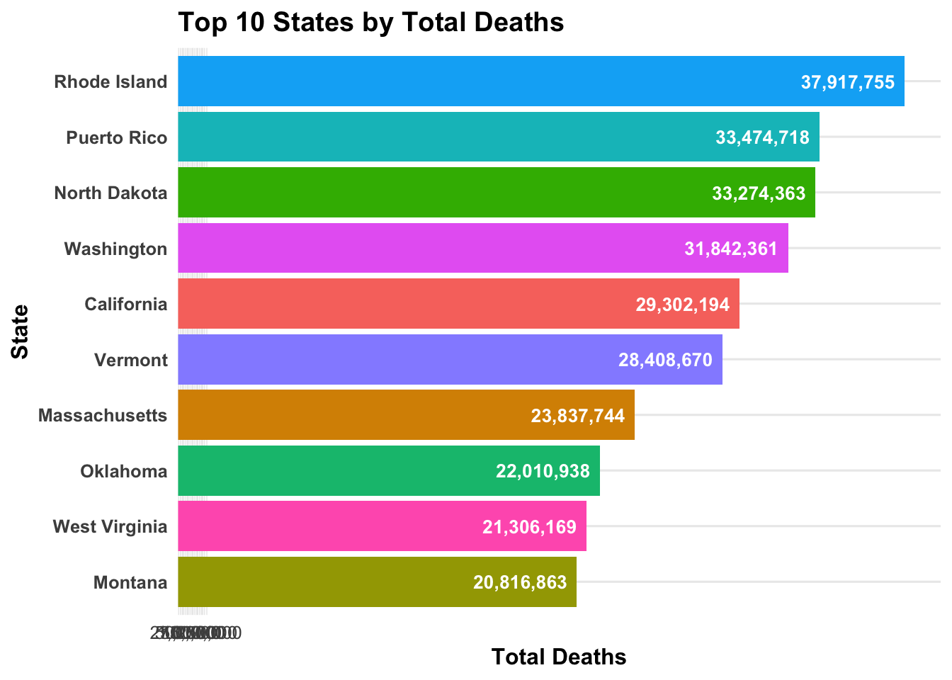
# Figure 1state_totals_MR <- syn_data_MR %>%filter(state !="United States") %>%group_by(state) %>%summarise(total_deaths =sum(total_deaths, na.rm =TRUE), .groups ="drop")# this gives us the top 10 states by total deaths, which we can plot in a horizontal bar chart.top10_MR <- state_totals_MR %>%arrange(desc(total_deaths)) %>%slice_head(n =10)# horizontal bar chart: states on y-axis, total_deaths on x-axis ggplot(top10_MR, aes(x =reorder(state, total_deaths), y = total_deaths, fill = state)) +geom_col() +geom_text(aes(label =comma(total_deaths)),hjust =1.1, # move text slightly inside barcolor ="white",fontface ="bold",size =3.5 ) +coord_flip() +# flip coordinates for horizontal barsscale_fill_hue() +scale_y_continuous(breaks =seq(0, max(top10$total_deaths, na.rm =TRUE), by =250000),labels = comma,expand =expansion(mult =c(0, 0.05)) ) +labs(title ="Top 10 States by Total Deaths",x ="State",y ="Total Deaths" ) +theme_minimal(base_size =12) +theme(plot.title =element_text(face ="bold"),axis.title.x =element_text(face ="bold"),axis.title.y =element_text(face ="bold"),axis.text.y =element_text(face ="bold"),legend.position ="none" )
Show the code
# Fits for synthetic datafit1_MR <-lm(covid_deaths ~ age_group, data = syn_data_MR)summary(fit1_MR)
Call:
lm(formula = covid_deaths ~ age_group, data = syn_data_MR)

Residuals:
    Min      1Q  Median      3Q     Max
  -1630   -1121   -1006    -756 1145931

Coefficients:
                           Estimate Std. Error t value Pr(>|t|)
(Intercept)                  976.73     311.63   3.134  0.00172 **
age_group1-4 years            63.12     438.27   0.144  0.88549
age_group15-24 years         147.88     440.45   0.336  0.73706
age_group18-29 years         -20.99     439.38  -0.048  0.96191
age_group25-34 years         549.08     438.29   1.253  0.21029
age_group30-49 years        -220.90     440.45  -0.502  0.61599
age_group35-44 years        -250.59     443.00  -0.566  0.57163
age_group45-54 years         211.52     440.97   0.480  0.63146
age_group5-14 years           58.07     441.65   0.131  0.89538
age_group50-64 years         351.00     442.65   0.793  0.42781
age_group55-64 years         142.96     444.48   0.322  0.74773
age_group65-74 years         -76.90     441.53  -0.174  0.86173
age_group75-84 years         290.23    2203.31   0.132  0.89520
age_group85 years and over   653.53     436.63   1.497  0.13446
age_groupAll Ages             52.43     444.07   0.118  0.90601
age_groupUnder 1 year        102.21     439.64   0.232  0.81616
---
Signif. codes:  0 '***' 0.001 '**' 0.01 '*' 0.05 '.' 0.1 ' ' 1

Residual standard error: 21150 on 69111 degrees of freedom
  (30873 observations deleted due to missingness)
Multiple R-squared:  0.0001314, Adjusted R-squared:  -8.557e-05
F-statistic: 0.6057 on 15 and 69111 DF,  p-value: 0.873
Show the code
fit2_MR <-lm(covid_deaths ~ race_origin, data = syn_data_MR)summary(fit2_MR)
Call:
lm(formula = covid_deaths ~ race_origin, data = syn_data_MR)

Residuals:
    Min      1Q  Median      3Q     Max
  -1653   -1088    -956    -865 1145812

Coefficients:
                                                                  Estimate
(Intercept)                                                            6.5
race_originNon-Hispanic American Indian or Alaska Native            1071.3
race_originNon-Hispanic Asian                                       1081.2
race_originNon-Hispanic Black                                        868.7
race_originNon-Hispanic More than one race                          1646.5
race_originNon-Hispanic Native Hawaiian or Other Pacific Islander    978.8
race_originNon-Hispanic White                                       1227.4
race_originTotal Deaths                                              949.0
race_originUnknown                                                   900.3
                                                                  Std. Error
(Intercept)                                                           7476.3
race_originNon-Hispanic American Indian or Alaska Native              7479.7
race_originNon-Hispanic Asian                                         7479.8
race_originNon-Hispanic Black                                         7479.8
race_originNon-Hispanic More than one race                            7479.7
race_originNon-Hispanic Native Hawaiian or Other Pacific Islander     7479.7
race_originNon-Hispanic White                                         7479.8
race_originTotal Deaths                                               7479.7
race_originUnknown                                                    7479.7
                                                                  t value
(Intercept)                                                         0.001
race_originNon-Hispanic American Indian or Alaska Native            0.143
race_originNon-Hispanic Asian                                       0.145
race_originNon-Hispanic Black                                       0.116
race_originNon-Hispanic More than one race                          0.220
race_originNon-Hispanic Native Hawaiian or Other Pacific Islander   0.131
race_originNon-Hispanic White                                       0.164
race_originTotal Deaths                                             0.127
race_originUnknown                                                  0.120
                                                                  Pr(>|t|)
(Intercept)                                                          0.999
race_originNon-Hispanic American Indian or Alaska Native             0.886
race_originNon-Hispanic Asian                                        0.885
race_originNon-Hispanic Black                                        0.908
race_originNon-Hispanic More than one race                           0.826
race_originNon-Hispanic Native Hawaiian or Other Pacific Islander    0.896
race_originNon-Hispanic White                                        0.870
race_originTotal Deaths                                              0.899
race_originUnknown                                                   0.904

Residual standard error: 21150 on 69118 degrees of freedom
  (30873 observations deleted due to missingness)
Multiple R-squared:  0.0001249, Adjusted R-squared:  9.15e-06
F-statistic: 1.079 on 8 and 69118 DF,  p-value: 0.3743
Wendling, T., Dumitras, S., Ogungbenro, K. et al. Application of a Bayesian approach to physiological modelling of mavoglurant population pharmacokinetics. J Pharmacokinet Pharmacodyn 42, 639–657 (2015). https://doi.org/10.1007/s10928-015-9430-4
Link to BayesPBPK-tutorial : https://github.com/metrumresearchgroup/BayesPBPK-tutorial